XAI: A Middleware for Scalable AI

Abdallah Salama, Alexander Linke, Igor Pessoa Rocha and Carsten Binnig

Data Management Lab, TU Darmstadt, Germany

Keywords:

Distributed Deep Learning, Machine Learning, Cloud Computing, Scalability.

Abstract:

A major obstacle for the adoption of deep neural networks (DNNs) is that the training can take multiple

hours or days even with modern GPUs. In order to speed-up training of modern DNNs, recent deep learning

frameworks support the distribution of the training process across multiple machines in a cluster of nodes.

However, even if existing well-established models such as AlexNet or GoogleNet are being used, it is still a

challenging task for data scientists to scale-out distributed deep learning in their environments and on their

hardware resources. In this paper, we present XAI, a middleware on top of existing deep learning frameworks

such as MXNet and Tensorﬂow to easily scale-out distributed training of DNNs. The aim of XAI is that data

scientists can use a simple interface to specify the model that needs to be trained and the resources available

(e.g., number of machines, number of GPUs per machine, etc.). At the core of XAI, we have implemented a

distributed optimizer that takes the model and the available cluster resources as input and ﬁnds a distributed

setup of the training for the given model that best leverages the available resources. Our experiments show

that XAI converges to a desired training accuracy 2x to 5x faster than default distribution setups in MXNet and

TensorFlow.

1 INTRODUCTION

Motivation: Deep Neural Networks (DNNs) have re-

cently seen a signiﬁcant adoption and are today driv-

ing the adoption of Machine Learning (ML) and Ar-

tiﬁcial Intelligence (AI) across a wide range of ap-

plication domains. The expressiveness of DNNs pro-

vides accurate solutions for many complex tasks such

as speech recognition, machine translation or image

understanding previously thought to be unsolvable by

machines, simply by observing large amounts of data.

A major obstacle for the adoption of DNNs, however,

is that the training of deep networks can take multiple

hours or days even with modern GPUs. Furthermore,

sizes of datasets and complexity of DNNs continu-

ously grow to solve even more complex tasks with

higher accuracy. This has the effect that the computa-

tional intensity and memory demands of deep learn-

ing increase further.

In order to speed-up training of modern DNNs on

large data sets, most of the deep learning frameworks

(such as Tensorﬂow (Abadi et al., 2016), MXNet

(Apache MXNet, 2018), or CNTK (Microsoft CNTK,

2018)) support the distribution of the training process

across multiple machines in a cluster of nodes. How-

ever, even if existing well-established models (such

as AlexNet, GoogleNet, or ResNet) are being used it

is still a challenging task for data scientists to imple-

ment scale-out distributed deep learning in their envi-

ronments.

The main reason is that data scientists must de-

cide on a multitude of low-level details (e.g., select-

ing how many parameter servers to use amongst many

other parameters) in order to distribute the training,

which have an effect on the overall scalability of

training DNNs. This often leads to a long and te-

dious trial-and-error process before the desired per-

formance advantages of distributing the training ac-

tually materialize (if at all). According to our own

experiences when using Tensorﬂow and MXNet as

well as based on discussions with other users of these

frameworks and experience reports (Sergeev and Del

Balso, 2018; O’Reilly Podcast, 2018), setting up a

distributed learning process for a new model architec-

ture can take days or weeks even for machine learning

experts.

Furthermore, there are many aspects, which make

the situation even worse. One major aspect is that the

trial-and-error procedure of ﬁnding an optimal setup

for scalable distributed training has to be repeated

over and over not only for every new model archi-

tecture but also when a new generation of hardware

(GPU, network, etc.) or even if a software version be-

comes available due to missing higher-level abstrac-

tions in those frameworks. This additionally turns the

maintenance of model training at scale into a tech-

nical debt that needs to be payed constantly (Sculley

et al., 2015).

Salama, A., Linke, A., Rocha, I. and Binnig, C.

XAI: A Middleware for Scalable AI.

DOI: 10.5220/0008120301090120

In Proceedings of the 8th International Conference on Data Science, Technology and Applications (DATA 2019), pages 109-120

ISBN: 978-989-758-377-3

109

Table 1: Popular Deep Neural Networks.

NETWORK # PARAMETERS DEPTH YEAR

ALEXNET 62,378,344 8 2012

VGG16 138,357,544 16 2014

GOOGLENET 6,797,700 22 2014

RESNET-50 25,636,712 50 2015

RESNET-152 60,344,232 152 2015

INCEPTION V3 23,851,784 159 2015

Contribution: In this paper, we present XAI, a mid-

dleware on top of existing deep learning frameworks

that enables data scientists to easily scale-out dis-

tributed training of DNNs. The aim of XAI is that

data scientists can use a simple interface to specify

the model that needs to be trained as well as the re-

sources available (e.g., number of machines, number

of GPUs per machine, etc.). Based on this input, XAI

automatically deploys the model on the available re-

sources in an optimal manner.

In order to enable scalable deep learning, XAI

comes with different components. At the core of

XAI, we have implemented a distributed optimizer

that takes the model and data as input and ﬁnds an op-

timal conﬁguration of the distributed training proce-

dure that maximizes throughput of the training proce-

dure for a given set of hyper-parameters (e.g., batch-

size and learning rate). In addition to the optimizer,

XAI comes with two more components: First, XAI

implements a component which automates the de-

ployment of the model based on the distribution pa-

rameters (e.g., number of parameter servers) deter-

mined by the optimizer. Currently, we have imple-

mented adapters to support Apache MXNet and Ten-

sorFlow as recent deep learning platforms and Ku-

bernetes and Slurm that are today being used typi-

cally in Cloud-based and HPC-based clusters. Sec-

ond, XAI additionally implements an adaptive execu-

tor component which not only monitors the available

resources (CPUs, GPUs, and network utilization) but

also adaptively changes the deployment if over- or

under-utilization of resources is detected.

In summary, we make the following contributions

in this paper: (1) We present XAI, a novel middleware

to simplify scalable distributed training that we plan

to open-source mid 2019. (2) We discuss the design

of a distributed optimizer which is a core component

of XAI to automatically ﬁnd an optimal deployment

strategy for a given model and available resources. (3)

We show in an extensive evaluation, that XAI can be

used to train different DNN architectures at scale and

support various possible deployments including dif-

ferent deep learning platforms, different cluster envi-

ronments, as well as different hardware generations

without hard-coding a new cost model for each new

setup.

Outline: The remainder of this paper is structured

as follows. Section 2 ﬁrst discusses the background

of distributed deep learning. Section 3 then gives an

overview of the architecture of XAI before we then

explain the details of the different components in Sec-

tions 4 to 6. The evaluation, in Section 7, shows the

result of using XAI to scale-out deep learning using a

variety of different workloads. Finally, we conclude

with an overview of the related work in Section 8 and

a summary of the ﬁndings and possible avenues of fu-

ture work in Section 9.

2 DEEP LEARNING

In this section, we give a brief overview of deep neural

networks (DNNs) and how typically distributed train-

ing works for DNNs.

2.1 Deep Neural Networks

DNNs represent a class of machine learning models

that has been rapidly evolving over the last couple of

years and have shown to be applicable to a wide area

of domains like image classiﬁcation, object detec-

tion, speech recognition or machine translation. The

ﬁrst approaches of simple neural networks, so called

feed-forward networks, were already published in the

1950’s (Rosenblatt, 1958) However, the accuracy of

those models was worse than classical machine learn-

ing methods (Minsky and Papert, 1969).

With increasing computational power and larger

datasets it was possible to train deeper neural net-

works (Hinton and Salakhutdinov, 2006) and outper-

form classical machine learning algorithms. One of

the ﬁrst breakthroughs was the accomplishment of

(Krizhevsky et al., 2012) with a neural network con-

taining eight layers. This Neural Network, so called

AlexNet, excelled at the ImageNet competition (Deng

et al., 2009) and achieved the highest accuracy un-

til then (Krizhevsky et al., 2012). To exemplify the

growth in complexity of DNNs in the last years, Ta-

ble 1 shows a selection of popular neural networks for

image classiﬁcation with their number of layers and

parameters.

2.2 Distributed Training

While the computational power and capacity of mod-

ern GPUs has been continuously growing (Ben-Nun

and Hoeﬂer, 2018), recent frameworks additionally

DATA 2019 - 8th International Conference on Data Science, Technology and Applications

110

support distributed training of DNNs to leverage the

capacity of GPUs across multiple machines.

Distributing the workload across multiple nodes,

however, involves splitting the training procedure

across multiple machines, which typically comes in

two forms for DNNs (Campos et al., 2017): First,

model-parallelism splits the model across machines

(e.g., based on its layers) and every node trains a part

of the model with the full dataset. Second, with data-

parallelism the datasets are split across workers and

every worker trains the full model but only using a

part of the data. While recent deep learning frame-

works support both schemes, this paper focuses on

data-parallelism, which has seen wider adoption in

practice than model-parallelism.

For data-parallelism, typically a centralized pa-

rameter server infrastructure is used to synchronize

the model across multiple machines (Dean et al.,

2012). The idea is that each worker node sends the

model parameters to the centralized parameters server

infrastructure, which merges the updates from differ-

ent workers and sends back the updated parameters

to the workers for the next mini-batch which is being

trained. To avoid that the centralized parameter server

infrastructure becomes a bottleneck, the parameters

can be sharded across multiple parameter servers.

A major challenge when using a centralized pa-

rameter server infrastructure for distributed training

is to balance computation and communication to best

leverage all resources (e.g., GPUs and the available

network) and enable scalability when more workers

with additional GPUs are being added. Deep learn-

ing frameworks therefore come with a variety of pa-

rameters that inﬂuence the ratio of computation and

communication such as model consistency (i.e., asyn-

chronous or synchronous updates (Jin et al., 2016)),

mini-batch size, but also the number of parameter

servers being used to shard the update load. If these

parameters are not chosen carefully, the overall scal-

ability is limited as we will show in our experimental

evaluation in Seciton 7.

3 SYSTEM OVERVIEW

XAI is built as a middleware on top of existing ma-

chine learning frameworks such as Apache MXNet

and TensorFlow. The purpose of XAI is to facilitate

the process of running deep learning training by in-

troducing a high-level interface, which hides the com-

plexity of deploying a DNN in a distributed manner.

Figure 1 shows the system architecture of XAI. In the

following, we brieﬂy discuss each component.

Job Monitor

Python

Library

Job Submission

Distributed

Optimizer

Hyper-

Parameter

Selection

Hyperparameter

Metadata

…

Distribution-

Parameter

Selection

Adaptive

Executer

Resource

Monitor

Script Generator

Re-

Conﬁguration

Workers Parameter Servers

Automatic

Deployment

Cluster

Environment

Scripts

Distributor

Execution

Delegator

Model and Data

Results / Resource Utilization

Train

Model

Model, Data, and Conﬁguration Results / Resource Utilization

Runtime Scripts

Conﬁguration

Results / Resource Utilization

Deep Learning Frameworks (Tensorﬂow, MXNet)

Cluster Manager

(Kubernetes, Slurm)

XAI

Client

XAI

Middleware

Existing

Infastructure

Figure 1: XAI System Architecture.

Client: XAI comes with a thin Python-based inter-

face that initiates the training job where the user only

has to specify the model (e.g., AlexNet), the data set

which is being used for the training procedure, and

the cluster metadata on which the training job will be

executed.

Additionally, the XAI client provides a simple in-

terface for monitoring the training results as well as

the resource utilization (e.g., of GPUs, network) on-

line and visually during training.

Distributed Optimizer: A major component of

XAI is the distributed optimizer that is able to ﬁnd

an optimal conﬁguration for a given DNN model and

data set (training and test data). An optimal conﬁg-

uration consists of the hyper-parameters that maxi-

mize the model accuracy as well as the distribution-

parameters (e.g., number of parameter servers) that

maximize the overall throughput in a distributed

setup. The main challenge to maximize the over-

all throughput is to estimate the network bandwidth

when running the training job in order to derive the

minimum number of parameter servers required to not

slow-down the training procedure. Section 4 explains

the details of the distributed optimizer of XAI.

Automatic Deployment: Given a conﬁguration

from the optimizer, the DNN model is then automat-

ically deployed in a cluster environment. A cluster

environment is deﬁned by the framework (e.g., Ten-

sorﬂow and MXNet) as well as the cluster manager

(e.g., Kubernetes and Slurm) that should be used for

executing the training job. Based on the conﬁgura-

tion and the given cluster environment, the XAI’s au-

tomatic model deployment component generates and

distributes the required training scripts to all nodes

(workers and parameter servers) and then delegates

the training to the available cluster manager (Slurm

or Kubernetes). Section 5 explains the details of the

model deployment of XAI.

XAI: A Middleware for Scalable AI

111

Adaptive Executor: The execution of a distributed

DNN training is monitored by an adaptive executor in

XAI. The purpose of the adaptive executor is to make

the execution more robust towards shared environ-

ments or non-optimal decisions by the optimizer. To

that end, the adaptive executor comes with a monitor-

ing component which continuously analyzes the uti-

lization of resources of all nodes (workers and param-

eter servers). Based on the monitored utilization, the

adaptive executor can change a running training job

by check-pointing the results of the last mini-batch

and continuing the training job with a new modiﬁed

conﬁguration (e.g., by increasing the number of pa-

rameter servers). Section 6 explains the details of the

adaptive executor of XAI.

4 DISTRIBUTED OPTIMIZER

In this section, we explain the details of our dis-

tributed optimizer, which is the core component of

XAI.

4.1 Overview of the Optimizer

As shown in the architecture of XAI in Figure 1,

the optimizer performs three steps that are executed

iteratively to explore the search space: (1) hyper-

parameter selection, (2) distribution-parameter selec-

tion, and then (3) model training. The overall aim of

the optimizer is to ﬁnd a model with high accuracy

with minimal runtime.

The idea behind the iterative search procedure is

that the ﬁrst step determines a set of hyper-parameters

(e.g., batch size, learning rate, etc.) that should be

used for training the next DNN in the next itera-

tion. In XAI, we currently implement a state-of-

the art approach based on selecting hyper-parameters

(Eggensperger et al., 2013), which is also available

in Auto-sklearn. This approach uses a random-forest-

based Bayesian optimization method SMAC to ﬁnd

the best instantiation of hyper-parameters. The ap-

proach additionally employs meta-learning to start

Bayesian optimization from good conﬁgurations eval-

uated on previous similar datasets and stores the re-

sults in our hyper-parameter Metadatabase. XAI also

uses this database to retrieve hyper-parameters for

next similar training job.

Once a set of hyper-parameters for the next iter-

ation is selected, the second step determines a set of

distribution-parameters to minimize the runtime (i.e.,

maximize the throughput) of the distributed training

procedure. This step, is not considered in the exist-

ing AutoML approaches which typically only focus

on hyper-parameter selection. The main contribution

of our optimization procedure is to combine the exist-

ing AutoML approaches for hyper-parameters selec-

tion with a selection of distribution-parameters which

minimize the runtime of distributed training. The de-

tails about the selection of distribution-parameters are

discussed next in Section 4.2.

Afterwards, once a set of hyper-parameters and

distribution-parameters are determined, the optimizer

trains the given DNN for a pre-deﬁned number of

epochs (using the automatic model deployment and

the adaptive execution component in XAI) and based

on the accuracy results it decides whether or not to

start a next iteration of optimization using the same

procedure as discussed before.

4.2 Distribution-parameter Selection

In the following, we describe our procedure for select-

ing a set of distribution-parameters to minimize the

runtime for a given set of hyper-parameters. In this

paper, we focus on distributed DNN training using

data-parallelism and a centralized parameter server

infrastructure with multiple servers where each hosts

a shard of parameters.

The two main distribution-parameters of interest

in our ﬁrst version of the optimizer are the number

of parameter servers being used as well as the up-

date strategy to synchronize the parameters between

workers and parameter servers. We picked the pa-

rameter server as a ﬁrst scheme that we support in

XAI since (a) it is widely used and supported by many

of the current distributed deep learning frameworks,

and (b) parameter servers have shown to be more efﬁ-

cient in wide range of possible deployments where no

dedicated hardware is available (e.g., InﬁniBand and

RDMA).

However, in future versions we also plan to

consider other distributed schemes including model-

parallelism as well as other approaches for data-

parallelism to distributed parameters (i.e., using repli-

cation approaches based on MPI to broadcast the pa-

rameters etc.).

When using data-parallelism and a centralized pa-

rameter server infrastructure, the aggregated network

bandwidth available between workers and parameter

servers is an important factor when it comes to scal-

ability. The main idea behind the optimizer is that

for a given number of workers, each having one or

multiple GPUs, we use a cost-model to estimate the

minimal number of parameter servers required to sus-

tain the update load. In order to do so, the opti-

mizer estimates the expected average network band-

width requirements between all workers and the cen-

DATA 2019 - 8th International Conference on Data Science, Technology and Applications

112

tralized parameter server for training a given DNN

architecture. Based on those estimated bandwidth-

requirements the number of parameter servers is de-

termined by simply dividing the required bandwidth

by the bandwidth each parameter server can provide

as we show later in Section 4.2.2.

4.2.1 Cost-model Calibration

Different from optimizers known from databases, the

optimizer in XAI does not use hard-coded cost-models

to estimate these values. Instead, in XAI we rely on

a short calibration phase that determines basic cost

model parameters experimentally. Using a calibra-

tion phase is typically not a problem for distributed

DNN training, since the training phase for one set of

hyper-parameters already takes hours or even days.

Compared to the time required for training, the time

required for the calibration phase is negligible.

The goal of the cost-model calibration is to de-

ﬁne the basic parameters such as the outgoing net-

work load each worker can produce as well as the

incoming network load a parameter server can con-

sume. Furthermore, a second parameter of interest is

the ratio of compute to communication time required

for a given DNN model architecture. This ratio is

an important parameter in our cost-based parameter

selection since it allows us to determine the number

of parameter servers required to minimize the overall

training runtime as we will see in the next subsection.

There are different factors which inﬂuence the ra-

tio of compute and communication time. First, hyper-

parameters such as the batch size or learning rate de-

termine the overall update load and thus the trans-

fer time. Second, the GPU and networking hardware

being used in the cluster setup play another impor-

tant role. Thus, calibration needs to be re-executed

when different hyper-parameters or a different hard-

ware setup is being used.

That way, our optimizer can determine an opti-

mal distributed setup for unseen DNN architectures

as well as new hardware generations without the need

of adapting a hard-coded cost models.

In order to ﬁnd out the ratio of compute and com-

munication time, the cost-Model calibration trains

ﬁrst the DNN with the given hyper-parameters on one

worker using all available GPUs without using a pa-

rameter server at all (i.e., all training is executed lo-

cally) for only a few mini-batches (i.e., we use 10

mini-batches at the moment to mitigate the effect of

outliers). The calibration phase then monitors the run-

time of the local training and divides it by the number

of batches. The time required to train one batch is

then used as an estimate to represent the total training

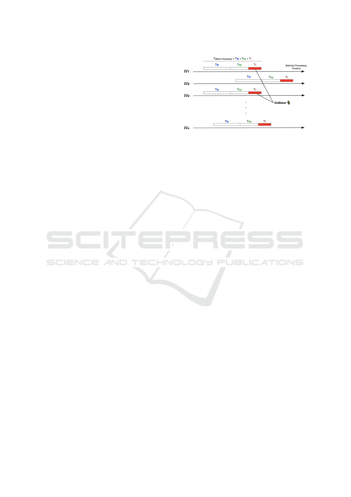
Figure 2: Collision Model of our Optimizer.

time including the forward propagation time T

f p

and

the backward propagation time T

Afterwards, the same procedure is performed us-

ing distributed setup with one worker and an increas-

ing number of parameter servers. We use our mon-

itoring capabilities of XAI to see when the outgoing

network bandwidth of the worker is saturated. The

purpose of this step is to ﬁnd the total batch process-

ing time T including the ideal transfer time T

if the

network is not a bottleneck. The difference between

the batch processing time with the local training is

used as an estimate for the transfer time to send the

weight updates from one worker over the network to

one parameter server; i.e., T

= T − (T

f p

+ T

). Fur-

thermore, based on this step of the calibration phase,

we can also identify the outgoing network bandwidth

load that one worker BW

can produce.

Finally, as a last step of the calibration phase, we

run the training in a distributed setup with one pa-

rameter server and an increasing number of workers.

Using our monitoring capabilities, we can thus deter-

mine the maximum network bandwidth BW

that a

parameter server is able to sustain.

4.2.2 Cost-based Parameter Selection

The goal of the cost-based parameter selection is to

ﬁnd the minimum number of parameter servers re-

quired to cover the network load generated by n work-

ers under different consistency models (asynchronous

and synchronous updates). In our current version,

we use asynchronous updates as a default while XAI

can also be conﬁgured to use synchronous training.

However, asynchronous updates have shown to pro-

vide an overall better runtime but might result in a

slower convergence. Modeling the dependency be-

tween throughput and convergence for asynchronous

and synchronous updates is left for future work.

Estimating the number of parameter servers re-

quired for synchronous updates is trivial. If we as-

sume that all workers send and receive data from pa-

rameter servers at the same time, then we can simply

XAI: A Middleware for Scalable AI

113

compute the required number of parameter servers as

n · BW

/BW

When using asynchronous parameter updates it is

more difﬁcult, since each worker sends its updates

independently. In the ideal case, if the communi-

cation of workers is not overlapping we would only

require BW

/BW

parameter servers independent of

the number of workers n being used. However, with

an increasing number of workers the likelihood that

two workers send/read parameters from a centralized

parameter server infrastructure at the same time in-

creases. In the following, we show how we can esti-

mate this likelihood.

If we have n workers and 1 parameter server, the

range of workers which are transferring data at the

same time can in general vary between 1 and n work-

ers. Figure 2 shows the basic idea of our collision

model that we use to estimate the collision likelihood

that m workers (where 1 < m ≤ n) transmit their pa-

rameters at the same time.

As basic input to estimate the likelihood that m out

of n workers collide, we use the following estimates

that we computed as a part of the calibration phase: T

which represents the total time to train a mini-batch

in one worker including the transfer time T

. Based

on these parameters, we can compute the probability

that a worker transfers data as:

(1)

If we look to the workers as being independent,

then the probability that any possible combination of

two workers (





) in a cluster with n workers are send-

ing data to a parameter server at the same time is de-

ﬁned by the following equation:

(n) =





)

(2)

This formula can be generalized to the probability

(n,m) that any possible combination of m workers

is sending at the same time.

(n,m) =





)

(3)

To calculate the probability that only one worker

sends data at any point of time during training, we use

equation 4:

(n,m = 1) = 1 −

∑

m=2





)

(4)

The purpose of calculating the overall likelihood

of collisions, is to estimate the expected bandwidth

that the workers could need to transmit param-

eter updates. The following equation deﬁnes how

to compute the expected bandwidth for a number of

workers based on the discussions before:

(n) =

∑

m=1

m · P

(n,m) · BW

(5)

After calculating the expected bandwidth E

(n)

for n workers, we can now estimate the number of the

parameters servers PS(n) required for n workers as

follows:

PS(n) =



(n)



(6)

In some cases when the transfer time T

is dom-

inating the batch processing time T , Equation 6 re-

sults in an overestimate of the parameter servers.

This problem is explained in (Math Pages, 2018),

which discusses the probability of intersecting inter-

vals. Based on their results, our equations above only

hold if T

n−1

. To solve this issue we extended our

cost model to cover this case. However, due to lack

of space and since this is only an exceptional case, we

will add the estimates for this case to an extended ver-

sion of the paper that we plan to publish as technical

report.

In our experiments in Section 7, we show that our

estimate based on Equation 6 results in optimal selec-

tion of parameter servers for an asynchronous model

updates.

5 AUTOMATIC MODEL

DEPLOYMENT

The aim of the automatic model deployment is that a

XAI can deploy the training of a given DNN in dif-

ferent cluster environments. Currently, XAI supports

the automatic deployment of a given DNN model us-

ing Tensorﬂow or MXNet as DNN frameworks and

Slurm or Kubernetes as cluster scheduler.

In the following, we brieﬂy outline the challenges

and ideas that we addressed when deploying a training

job on Slurm or Kubernetes respectively.

5.1 Deployment using Slurm

A main challenge when executing MXNet or Tensor-

ﬂow in a Slurm-based environment is that resources

(i.e., workers and parameter servers) must be mapped

to physical resources (i.e., nodes) after a training job

is deployed.

This departs from most DNN frameworks, which

require a static assignment of resources before start-

ing a training job. To actually start a distributed train-

ing job in Tensorﬂow or MXNet it is necessary to

provide the host addressees of the different nodes and

their roles (workers and parameter servers) in a clus-

ter speciﬁcation.

DATA 2019 - 8th International Conference on Data Science, Technology and Applications

114

When using Slurm, this so called cluster speciﬁ-

cation can only be determined at runtime after the job

is deployed in a cluster. We therefore generate startup

scripts that dynamically create a cluster speciﬁcation

for each node being selected by Slurm.

5.2 Deployment using Kubernetes

The automatic deployment component also supports

Kubernetes, by automatically generating the proper

YAML-scripts for all the so called pods that will be

created on each node in a cluster. The challenges are

similar to the Slurm environment.

To dynamically deploy workers and parameter

servers, our deployment component automatically

creates internal Kubernetes services for each pod, so

that they can communicate through the pod addresses.

A training job receives at startup a pool of pod ad-

dresses as an argument that identiﬁes which pods are

participating in the training and who is taking over

role of being a parameter server or a worker.

6 ADAPTIVE EXECUTOR

The main component of the adaptive executor is the

resource monitoring component. This component

records important metrics about the hardware perfor-

mance of individual nodes (i.e., workers and parame-

ter servers) to track possible bottlenecks. The identi-

ﬁcation of bottlenecks on a high level helps to quickly

investigate the problem more accurately with speciﬁc

tools or directly adapt the DNN training deployment

to utilize all resources uniformly.

The currently selected metrics include the CPU

utilization, main memory consumption, in- and out-

going network trafﬁc as well as GPU load and GPU

memory consumption. Even during developing XAI,

the monitoring tool has often helped us to directly

identify if we are running into a network or GPU bot-

tleneck or to detect a skew on the parameter servers.

The monitoring component is implemented as a

python program which runs on one CPU core in par-

allel to the DNN training process, records the given

metrics, and writes them to a log ﬁle. The logs from

all nodes are continuously collected, transformed and

analyzed, so that the training can be adapted accord-

ing to the monitoring results and, for instance, scale-

in or scale-out the parameter server infrastructure if

more resources are needed. For manual investigation,

we additionally provide a service for visualizing the

analyzed data using the before-mentioned metrics.

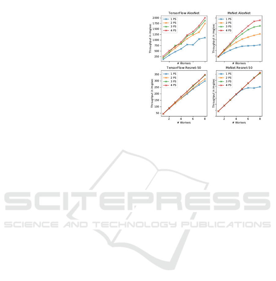
Figure 3: Throughput Analysis for AlexNet and ResNet-50

using TensorFlow on the HPC Cluster with Asynchronous

Training.

7 EXPERIMENTAL EVALUATION

In our experimental evaluation, we have trained neu-

ral networks in a distributed way on different clusters

and deep learning frameworks using various hyper-

and distribution-parameters. To give an overview and

back up the need for a cost-based optimizer in XAI,

the following sections will ﬁrst illustrate how that dif-

ferent parameters signiﬁcantly inﬂuence the perfor-

mance of the DNN training. Furthermore, we also

show the efﬁciency of our optimizer to select an op-

timal set of parameters as well as interesting ﬁndings

that where eable to derive from using our monitoring

component.

Setup and Workloads: In all our experiments, we

have used the two cluster setups as shown in Table 2.

We have chosen two different setups: one setup on an

HPC-cluster with a fast network connection and one

setup using an AWS-cluster with a slower network

connection. Furthermore, both setups differ also in

the GPU generation being used.

The DNN models we have used for the evalua-

tion are listed in Table 1. These DNNs have been

used over the last years for image classiﬁcation rep-

resenting different model architectures. We believe

that our ﬁndings and cost models can also be general-

ized to other domains using different model architec-

tures (e.g., sequence-to-sequence models for machine

translation). Showing this, however, is part of our fu-

ture work.

Furthermore, in our evaluation we only show the

effects of selecting different parameters on the overall

XAI: A Middleware for Scalable AI

115

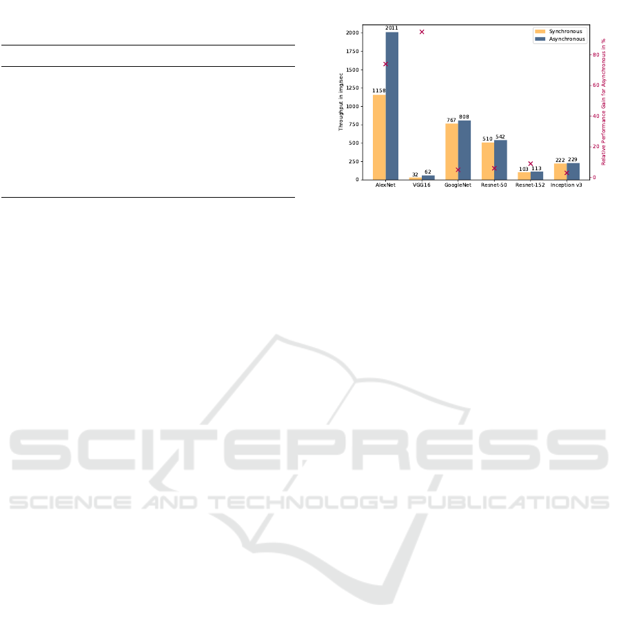
Table 2: Machine Conﬁguration in Different Clusters.

CLUSTER HPC AWS (P2.XLARGE)

CPU 2X XEON E5-2670 4X VCPU

RAM 32 GBYTE 61 GBYTE

BANDWITH 20 GBIT/S 1.3 GBIT/S

GPU 2X TESLA K20X 1X TESLA K80

OS CENTOS 7 UBUNTU 16.02

TENSORFLOW 1.10 1.10

MXNET 1.2.1 N.A.

CUDA 9.0 9.0

CUDNN 7.1.3 7.1.3

throughput and not on the model accuracy. The reason

is that the main contribution of our optimizer is the

cost-based model to ﬁnd an optimal distributed setup,

which aims to minimize runtime. Consequently, in

all our experiments we also used only synthetic data

sets; i.e., images are represented as in-memory arrays

with random values, to avoid running into bottlenecks

(e.g., I/O limitations of shared ﬁle systems) not rele-

vant for our evaluations.

7.1 Exp 1: Throughput Analysis

We have empirically evaluated several hundreds of

distributed setups to show the sensitivity of the train-

ing throughput from different parameters. The results

clearly justify the need for a calibration phase to make

XAI not only independent of the DNN architecture but

also independent of the framework being used as well

as the underlying hardware. In the following sections

we summarize the most important ﬁndings.

7.1.1 Different Frameworks

By training DNNs on different frameworks, we saw

a difference in terms of throughput when using dif-

ferent Deep Learning Frameworks like TensorFlow

or MXNet. In Figure 3, the upper plots show how

the training throughput in TensorFlow for training

AlexNet using asynchronous model consistency can

achieve a higher throughput with a lower amount of

parameter servers (PS) than with MXNet. What is

not shown in the plots, is that in synchronous mode,

TensorFlow performs up to 30% worse than MXNet

with a higher number of parameter servers, whereas

TensorFlow still outperforms MXNet with a small

amount of parameter servers.

In the lower two plots of Figure 3, we addition-

ally see that when using another DNN (ResNet-50)

there is no big difference between the two frame-

works. However, the previous observation also ap-

plies here. MXNet needs more parameter servers for

scaling-out. This is indicated by the 1 PS line in

the lower right subplot, which stops increasing at a

Figure 4: Throughput Analysis in TensorFlow for different

DNNs with 8 Worker and 4 Parameter Servers on the HPC

Cluster.

throughput of around 250 images per second. The

general ability to achieve a better scale-out with fewer

parameter servers in ResNet-50 in both frameworks is

due to a higher computational requirements for train-

ing this DNN. As a result the ratio of communication

to computation shifts to a less network-bound situa-

tion.

7.1.2 Different DNNs

Figure 4 illustrates the throughput difference when

training the different DNNs mentioned in Table 1. It is

noticeable that the difference in throughput is related

to the difference in computational complexity of the

DNNs, which is not the same as the number of param-

eters a DNN has but also depends on the types of lay-

ers used. As a result, for some DNNs with low com-

putational complexity, the throughput is much higher

if a fast network interconnection is being used be-

cause the ratio of computation over communication

shifts and makes the overall training network-bound.

7.1.3 Different Consistency Models

In this experiment, we analyze the effect of differ-

ent consistency models on the overall throughput as

shown in Figure 4. For some DNNs like AlexNet

and VGG16, we can see an high increase for asyn-

chronous over synchronous training of up to 80%,

shown by the red markers in Figure 4. This is caused

by the high amount of parameters of those networks,

while the depth (i.e., number of layers) is compara-

bly low compared to other DNNs. As a result, we can

see that the performance gains of asynchronous train-

ing over synchronous training depend heavily on the

DNN architecture.

7.1.4 Different Batch Sizes

Figure 5 shows that the mini-batch size inﬂuences

the throughput during distributed training. The x-axis

DATA 2019 - 8th International Conference on Data Science, Technology and Applications

116

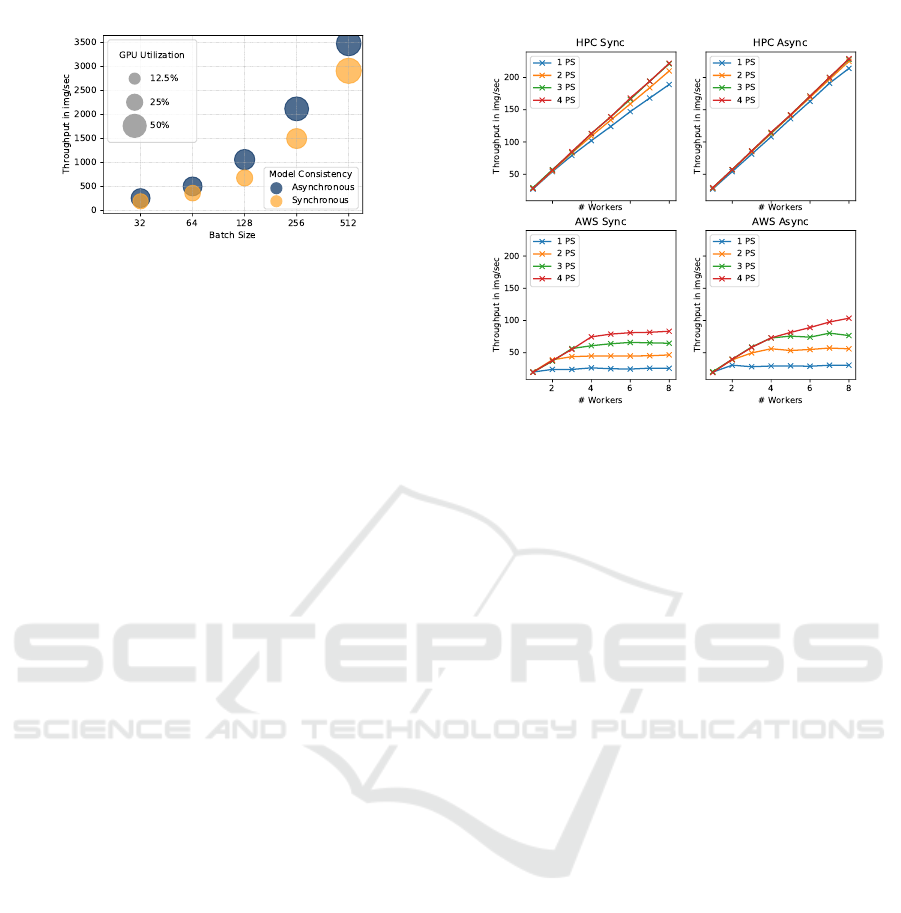
Figure 5: Effect of Batch Size on the Throughput for train-

ing AlexNet with 8 Workers and 1 parameter server on the

HPC Cluster.

shows the batch size for a single worker on a loga-

rithmic scale and the y-axis shows the throughput. In

this experiment, we only show the result of AlexNet.

For this DNN, the throughput scales almost linearly

with an increasing in mini-batch size. What we can

also see is that an increase in mini-batch size leads to

a higher GPU utilization of the workers, since a sin-

gle worker processes more images per batch such that

the ratio between communication over computation

decreases. It is further noticeable that asynchronous

training performs on average 38% better than syn-

chronous training.

7.1.5 Different Cluster Environments

In this experiment, we show the effects of using dif-

ferent cluster setups (HPC vs. AWS). The lower plots

in Figure 6 indicate that the DNN training on AWS

with a comparably slow network connection (see Ta-

ble 2) shows effects of network congestion. The in-

crease of parameter servers for AWS thus helps to

mitigate the congestion to a certain extend and bet-

ter scale out. The DNN training on the HPC cluster

(upper plots in Figure 6) on the other shows a much

better scalability with fewer parameter servers. Only

in the case of synchronous training, we also see that

network becomes a bottleneck when using only one

parameter server for 8 workers. This originates from

network peak requirements in synchronous training,

since all workers send their updates and receive new

parameters (almost) simultaneously.

7.2 Exp 2: Accuracy of Optimizer

The goal of this experiment is to show the accuracy

of our cost model. To show that, we executed the dis-

tributed training procedure with a varying number of

workers where we ﬁrst manually varied the number of

parameter servers and then compared it to the training

in XAI where our optimizer determined the number

of parameter servers for a given number of workers.

Figure 6: Training of Inception v3 on different Clusters.

The idea is that the optimizer neither under-estimates

nor over-estimates the number of parameter servers

required to sustain the load of the workers.

In the following we show the results when apply-

ing our cost model not only for different DNN mod-

els, but also when using deep learning frameworks

as well as different cluster setups. However, due to

space limitations, we only show the results of the cost

model for asynchronous training, which is also more

challenging to model as explained in Section 4.

Figure 7 shows the result of training ResNet-50

on the HPC and the AWS clusters using TensorFlow.

The goal is to show the accuracy of the cost model

for different clusters using different hardware setups.

The red line shows the result of our cost model where

each point is annotated with the parameter servers that

our model predicted. As we see from the plot, our

cost model predicts the minimal number of parame-

ters servers that allows us to scale-out almost linearly

(i.e., it neither under- nor over-estimates the number

of parameter servers required). For example, for the

plot on the right hand side, we can see that the cost

model suggests to use 5 parameter servers for 4 work-

ers. Using more parameter servers would not increase

the throughput but using less than 5 servers would

signiﬁcantly decrease the overall throughput. What

is also interesting is that in the HPC cluster (left hand

side), where we have high network bandwidth, the op-

timizer in general recommends a fewer number of pa-

rameters servers compared to training the same DNN

on the AWS cluster (right hand side) where we have

only a slow network.

Figure 8 shows the result of training ResNet-

50 and AlexNet on the HPC cluster using Apache

MXNet. The goal is to show the accuracy of the cost

model for DNNs with a different computational com-

XAI: A Middleware for Scalable AI

117

Figure 7: Accuracy of the Optimizer for Different Clusters.

Figure 8: Accuracy of the Optimizer in Different DNNs.

plexity. In ResNet-50, our optimizer recommends to

use 2 parameters servers if up to 6 workers are be-

ing used. If we look to the throughput for 2 work-

ers, we can easily see that 2 parameters servers is

an optimal choice because using 3 or 4 parameters

servers would not increase the throughput. Moreover,

in AlexNet where the number of model parameters is

higher as for ResNet-50, the likelihood of collisions

(i.e., two workers send/receive their parameters at the

same time) is also higher. Thus, our optimizer selects

to use more parameters servers for the same number

of workers.

7.3 Exp 3: Resource Monitoring

The resource monitoring component provides infor-

mation about several metrics for each node of the

cluster as explained in Section 6. This component is

very helpful to identify unexpected behaviors during

training and helped us to point out potential bottle-

necks.

For instance, Figure 9 shows the monitored net-

work data received for the parameter servers dur-

ing the training of AlexNet when using 4 parame-

ter servers and 5 workers. In the upper plot, we see

that the network utilization for parameter servers (PS)

2 and 3, represented by green and orange lines, are

much higher, while the network utilization for param-

eter servers 1 and 4 is much lower. This information

led us to investigate how the parameters of AlexNet

were distributed among the four parameter servers.

The reason turned out to be skew in the way how

weights where distributed to parameter servers.

Further investigations led us to the following ﬁnd-

Figure 9: Network Data received by Parameter Servers with

and without Skew.

ings. AlexNet has three fully-connected layers: Two

with 4096 neurons each and one with only 1000 neu-

rons (Krizhevsky et al., 2012). Since each fully-

connected layer is one big operation in the compu-

tation graph, the load balancer of Tensorﬂow was as-

signing the parameters in a layer-wise manner to pa-

rameter servers. This layer-wise assignment was then

causing the skew on the network and consequently re-

ducing the overall training performance.

To solve the issue, we introduced a new partitioner

for AlexNet to split the layers in equal sized parts

according to the number of parameters servers, thus,

sharding the network load equally across servers. The

results after using our own partitioner for AlexNet can

be seen in the lower plot of Figure 9. As a main re-

sult, we see that the network load is better distributed

across all parameter servers and the overall training

time is thus reduced.

7.4 Exp 4: Effectiveness of XAI

XAI aims to execute a distributed job with highest

throughput that can be obtained out of a cluster set-

tings. This experiment shows the resulting effective-

ness of XAI by picking the optimal distribution strat-

egy and thus converging to a comparable accuracy 2x

faster than a default conﬁguration. Figure 10 shows

two similar asynchronous training jobs with 5 work-

ers to train AlexNet using TensorFlow on an AWS

cluster with and without XAI. By using the default

conﬁguration of TensorFlow (1 parameter server), the

training time was 2x slower than the training time

with XAI. The cost model optimizer in XAI recom-

mended to deploy 5 parameter servers.

DATA 2019 - 8th International Conference on Data Science, Technology and Applications

118

Figure 10: Effectiveness of the Cost Model Optimizer.

8 RELATED WORK

In this section, we discuss related work. We ﬁrst fo-

cus on recent systems and libraries that have a similar

goal as XAI to enable scalable AI. Afterwards, we dis-

cuss the broader area of automated machine learning

(AutoML) which is also relevant for this paper.

Scalable AI: Many recent deep learning frame-

works such as TensorFlow (Abadi et al., 2016),

MXNet (Apache MXNet, 2018), or CNTK (Microsoft

CNTK, 2018)) support the distribution of the train-

ing process across multiple machines in a cluster of

nodes. However, even if existing well-established

models (such as AlexNet, GoogleNet, or ResNet) are

being used it is still a challenging task to efﬁciently

scale-out distributed deep learning.

A system that takes similar approaches as XAI

to simplify the distributed training of DNNs with

is Horovod (Sergeev and Del Balso, 2018). How-

ever, there are major differences between XAI and

Horovod. First, Horovod is currently only support-

ing TensorFlow as a framework while XAI is built as

a middleware and can support different deep learning

frameworks. Second, XAI comes with an optimizer

which automatically deﬁnes the optimal number of

parameter servers which has to be manually tuned in

Horovod.

Another direction to scale out deep learning more

efﬁciently is to provide libraries that allow deep learn-

ing frameworks to implement a more efﬁcient com-

munication stack. One example, is the Intel Machine

Learning Scaling Library (MLSL) (Sridharan et al.,

2018). MLSL uses an implementation of the MPI

allreduce primitive to make communication more ef-

ﬁcient. Furthermore, MLSL also comes with some

adaptive execution strategies to better overlap com-

putation and communication. All these optimizations

are orthogonal to the goals of XAI and could be inte-

grated into any of the supported frameworks of XAI.

Another work which is relevant to XAI is (Omni-

Vore) (Hadjis et al., 2016), while (OmniVore) is an

optimizer for multi-device training, however, it works

as a separate system. The major difference is that XAI

is a middleware on top of existing systems and it is de-

signed to support different cluster conﬁgurations. The

ﬁnal target of XAI is to smartly and fully blackboxing

the distributed training job.

Automated Machine Learning: There have been

several attempts to automate machine learning to

make it more accessible. However, these approaches

typically concentrate on hyper-parameter selection

and not on the complete automated deployment of dis-

tributed machine learning as we do in XAI. One no-

table example is Auto-Weka (Thornton et al., 2013).

Auto-WEKA aims to automate the use of Weka (Ma-

chine Learning Group at the University of Waikato,

2018) by applying recent derivative-free optimization

algorithms, in particular Sequential Model-based Al-

gorithm Conﬁguration (SMAC) (Hutter et al., 2011),

to the hyperparameters tuning problem; a small sub-

problem of XAI. Furthermore, there are also Cloud

services like Google AutoML (Google AutoML,

2018). These services, however, are often only usable

in a limited number of scenarios as they signiﬁcantly

restrict the type of models that can be trained. More-

over, cloud services often enforce other limits such as

a maximum training data-size.

9 CONCLUSIONS

In this paper, we presented XAI, a middleware on

top of existing deep learning frameworks (Apache

MXNet and Tensorﬂow) to easily scale-out dis-

tributed training of DNNs. At the core of XAI, we

have implemented a distributed optimizer that takes

the model and the available cluster resources as input

and ﬁnds an optimal distributed setup of the training

procedure. In the ﬁrst version of XAI, we only sup-

port distributed training using data-parallelism with a

centralized parameter server. In future, we will ex-

tend XAI to also support not only other frameworks

but also other forms of data-parallelism within those

frameworks (e.g., by replicating the parameters). An-

other interesting route would be to include automatic

model-parallelism in XAI as well.

REFERENCES

Abadi, M. et al. (2016). Tensorﬂow: A system for large-

scale machine learning. In 12th USENIX Sympo-

sium on Operating Systems Design and Implementa-

XAI: A Middleware for Scalable AI

119

tion, OSDI 2016, Savannah, GA, USA, November 2-4,

2016., pages 265–283.

Apache MXNet (2018). Apache MXNet. https://mxnet.

apache.org/. Accessed: 2018-09-28.

Ben-Nun, T. and Hoeﬂer, T. (2018). Demystifying Parallel

and Distributed Deep Learning: An In-Depth Concur-

rency Analysis. CoRR, abs/1802.0.

Campos, V., Sastre, F., Yag

ues, M., Bellver, M., Gir

o-I-

Nieto, X., and Torres, J. (2017). Distributed training

strategies for a computer vision deep learning algo-

rithm on a distributed GPU cluster. Procedia Com-

puter Science, 108:315–324.

Dean, J., Corrado, G., Monga, R., Chen, K., Devin, M.,

Mao, M., Senior, A., Tucker, P., Yang, K., and Le,

Q. V. (2012). Large scale distributed deep networks.

Advances in Neural Information Processing Systems,

pages 1223–1231.

Deng, J., Dong, W., Socher, R., Li, L.-J., Kai Li, and Li

Fei-Fei (2009). ImageNet: A large-scale hierarchical

image database. In 2009 IEEE Conference on Com-

puter Vision and Pattern Recognition, pages 248–255.

IEEE.

Eggensperger, K., Feurer, M., Hutter, F., Bergstra,

J., Snoek, J., Hoos, H., and Leyton-Brown, K.

(2013). Towards an empirical foundation for assessing

bayesian optimization of hyperparameters. In NIPS

workshop on Bayesian Optimization in Theory and

Practice.

Google AutoML (2018). Google AutoML.

https://cloud.google.com/automl/. Accessed: 2018-

09-28.

Hadjis, S., , Zhang, C., Mitliagkas, I., et al. (2016). An

optimizer for multi-device deep learning on cpus and

gpus. In CoRR, page abs/1606.04487.

Hinton, G. E. and Salakhutdinov, R. R. (2006). Reducing

the dimensionality of data with neural networks. Sci-

ence (New York, N.Y.), 313(5786):504–7.

Hutter, F. et al. (2011). Sequential model-based optimiza-

tion for general algorithm conﬁguration. In Proceed-

ings of the 5th International Conference on Learning

and Intelligent Optimization, LION’05.

Jin, P. H., Yuan, Q., Iandola, F., and Keutzer, K. (2016).

How to scale distributed deep learning? CoRR.

Krizhevsky, A., Sutskever, I., and Hinton, G. E. (2012). Im-

ageNet Classiﬁcation with Deep Convolutional Neu-

ral Networks. Advances In Neural Information Pro-

cessing Systems, pages 1–9.

Machine Learning Group at the University of Waikato

(2018). Weka 3: Data Mining Software in Java.

http://www.cs.waikato.ac.nz/ml/weka/. Accessed:

2018-09-28.

Math Pages (2018). Probability of intersecting inter-

vals. http://www.mathpages.com/home/kmath580/

kmath580.htm. Accessed: 2018-09-24.

Microsoft CNTK (2018). The Microsoft Cognitive

Toolkit. https://www.microsoft.com/en-us/cognitive-

toolkit/. Accessed: 2018-09-28.

Minsky, M. and Papert, S. (1969). Perceptrons; an intro-

duction to computational geometry. MIT Press.

O’Reilly Podcast (2018). How to train and deploy deep

learning at scale. https://www.oreilly.com/ideas/how-

to-train-and-deploy-deep-learning-at-scale/. Ac-

cessed: 2018-09-28.

Rosenblatt, F. (1958). The perceptron: A probabilistic

model for information storage and organization in the

brain. Psychological Review, 65(6):386–408.

Sculley, D. et al. (2015). Hidden technical debt in machine

learning systems. In Advances in Neural Information

Processing Systems 28: Annual Conference on Neural

Information Processing Systems 2015, December 7-

12, 2015, Montreal, Quebec, Canada, pages 2503–

2511.

Sergeev, A. and Del Balso, M. (2018). Horovod: fast and

easy distributed deep learning in TensorFlow. CoRR.

Sridharan, S., Vaidyanathan, K., Kalamkar, D., Das, D.,

Smorkalov, M. E., Shiryaev, M., Mudigere, D.,

Mellempudi, N., Avancha, S., Kaul, B., and Dubey,

P. (2018). On Scale-out Deep Learning Training for

Cloud and HPC. CoRR, pages 16–18.

Thornton, C. et al. (2013). Auto-weka: combined selec-

tion and hyperparameter optimization of classiﬁcation

algorithms. In SIGKDD, pages 847–855.

DATA 2019 - 8th International Conference on Data Science, Technology and Applications

120

REFERENCES

Abadi, M. et al. (2016). Tensorflow: A system for large-