Clustering-based Model for Predicting Multi-spatial Relations in Images
Brandon Birmingham and Adrian Muscat
Department of Communications and Computer Engineering, University of Malta, Msida MSD 2080, Malta
Keywords:
Spatial Relations, Image Understanding, Multi-label Learning, Clustering, Computer Vision, Natural
Language Processing.
Abstract:
Detecting spatial relations between objects in an image is a core task in image understanding and grounded nat-
ural language. This problem has been addressed in cognitive linguistics through the development of template
and computational models from controlled experimental data using 2D or 3D synthetic diagrams. Further-
more, the Computer Vision (CV) and Natural Language Processing (NLP) communities developed machine
learning models for real-world images mostly from crowd-sourced data. The latter models treat the problem
as a single-label classification problem, whereas the problem is inherently a multi-label problem. In this paper,
we learn a multi-label model based on computed spatial features. We chose to implement the model using a
clustering-based approach since, apart from predicting multi-labels for a given instance, this method would
allow us to get deeper insights into how spatial relations are related to each other. In this paper, we report our
results from this model and a direct comparison with a Random Forest single-label classifier is presented. The
proposed model generally shows that it outperforms the single-label classifier even when considering the top
four prepositions predicted by the single-label classifier.
1 INTRODUCTION
Image understanding not only requires the detection
of objects depicted in an image but also the pre-
diction of spatial relationships between relevant ob-
jects. The latter sub-task, which is the focus of this
paper, plays an important role in image captioning
models as well as in robotic applications which in-
volve human-to-robot interaction and vice-versa. Pre-
dicting the spatial relation between objects is a non-
trivial task because the problem is (a) an inherently
multi-label problem, i.e., there may be more than
one relation that is applicable to a given context, and
(b) human beings are not consistent in the choice
of an appropriate relation (Muscat and Belz, 2017).
This inconsistency results from the selective nature
of near-synonym spatial relations, which is evident in
cases such as those involving two objects placed at
a lower level from each other and thus described by
one of the following equally plausible prepositions:
{“under”, “underneath”,“beneath”, “below”}. As an
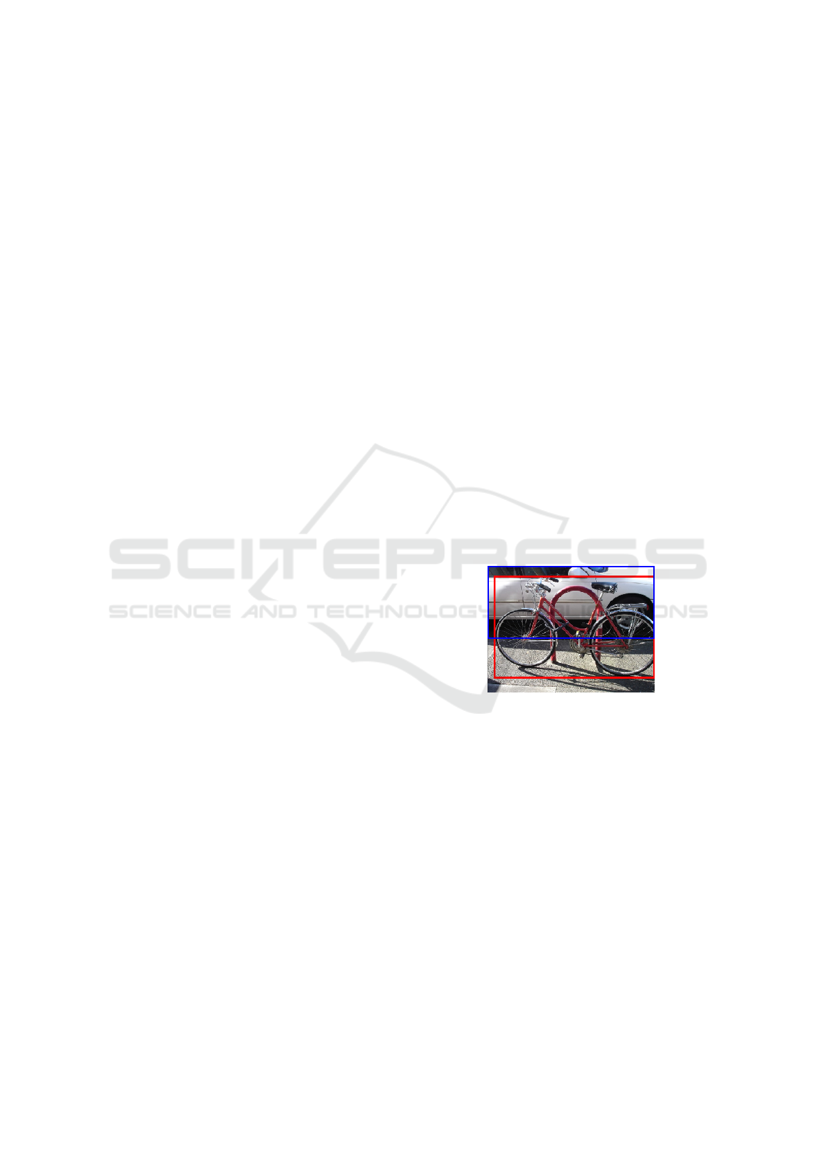
other example, the set of prepositions: next to, in front
of, along, and near can be used to describe the spatial
relationship between the bicycle and the car which are
illustrated in Figure 1.
This makes it inherently more challenging for su-
pervised learning-based models to recognise single
Figure 1: Example of multi-spatial relations between two
objects enclosed in bounding boxes: The bicycle is {next
to, in front of, along, near} the car.
label relations (class labels) for a given pair of ob-
jects. Traditional supervised learning attempts to clas-
sify the spatial orientation between two objects by as-
sociating feature vectors with single class labels. For-
mally, these models are trained to learn the function
f : X → Y , where X and Y represent the instance and
label spaces respectively. Instance and label training
pairs found in set D = {(x
i
,y
i
)|1 ≤ i ≤ m} are used
to automatically learn the semantic relationship be-
tween each x
i
∈ X and y
i
∈ Y , with the fundamen-
tal assumption that each instance belongs to a single
class concept (Zhang and Zhou, 2014). While consid-
ering the multi-label nature of spatial relation classi-
fication, a direct solution which addresses the afore-
mentioned difficulties is to cast spatial relation recog-
Birmingham, B. and Muscat, A.
Clustering-based Model for Predicting Multi-spatial Relations in Images.
DOI: 10.5220/0008123601470156
In Proceedings of the 16th International Conference on Informatics in Control, Automation and Robotics (ICINCO 2019), pages 147-156
ISBN: 978-989-758-380-3
Copyright
c
 2019 by SCITEPRESS – Science and Technology Publications, Lda. All rights reserved
147

nition as a multi-label classification problem, by as-
signing a set of appropriate labels (prepositions) for
each instance (Tsoumakas and Katakis, 2007). For
a given space X = ℜ
d
denoting each d-dimensional
feature vector per instance, and Y = {y
1
,y
2
,. .. y
q
}
which represents the label space with q distinct class
labels, multi-label learning aims to infer a function h :
X → 2
q
from the multi-label training data D. Multi-
label pairs are represented by (x
i
,y
i
), where x
i
is a d-
dimensional feature vector, while y
i
⊆ Y is the corre-
sponding set of associated labels. The learned multi-
label model h(·) is then applied to predict the set of
class labels h(x
i
) ⊆ Y for a given unseen x
i
∈ X.
Whilst also catering for the exponentially large
output space
1
involved in multi-label learning, in this
paper we are interested in studying (a) to what extent
we can generate multi-label models from limited data
and (b) what these models can tell us about the appli-
cation of multiple, but equally plausible prepositions
given a configuration. For these two reasons, we used
an unsupervised clustering method to provide results
from which we can use to build a multi-label model
designed to:
• Cluster spatial relations based on their feature
vectors in an unsupervised way.
• Analyse the preposition distribution found within
each cluster by making use of the labelled data.
• Classify unseen instances by finding the closest
cluster and output the predominant prepositions
found within the same cluster.
• Calculate the similarity between prepositions by
comparing their distribution across all clusters.
This section motivated the study and introduced
the problem. The rest of the paper is organised as fol-
lows. Section 2 presents an overview of related work
and Section 3 describes the dataset and features used
in this study. The experiment carried out is described
in Section 4 and is followed by Section 5 which dis-
cusses the results. The paper is concluded in Section 6
with a discussion and a look at the future direction.
2 RELATED WORK
In the psycho- and cognitive-linguistics literature,
the multi-label spatial recognition problem was
mainly addressed by the development of spatial tem-
plates (Logan and Sadler, 1996) and computational
models (Regier and Carlson, 2001), whilst the choice
for the “most” appropriate preposition was tackled
1
In theory, a multi-label problem having q = 17 distinct
labels results in 2
17
= 131, 072 possible output sets.
by considering the minimum cognitive load (least ef-
fort) in choosing an appropriate relation (Kelleher and
Kruijff, 2005). Such works were based on data gath-
ered from controlled experiments, using 2D and 3D
synthetic diagrams, where humans were asked to rate
the acceptability of a given preposition depicted in a
given configuration. Early models concentrated on
the geometric features that predict prepositions. How-
ever, further work emphasized the language and geo-
metrical bias of prepositions (Carlson-Radvansky and
Radvansky, 1996; Coventry et al., 2001; Dobnik and
Kelleher, 2014), and other work studied how percep-
tual features, such as occlusion, modify the spatial
templates (Kelleher et al., 2011).
The prediction of spatial relations is even more
difficult when images of the physical world are con-
sidered. Sadeghi and Farhadi (2011) were probably
the first to deal directly with relation detection in real-
world images and treated the problem as object detec-
tion. This method does not scale because of the large
number of unique meaningful relations that exist. The
obvious way is to compute spatial properties in addi-
tion to language and visual features. Two approaches
are considered when dealing with features obtained
from images, (a) methods based on image features
learnt via deep neural networks, mainly convolutional
neural networks (CNNs) (Lu et al., 2016; Dai et al.,
2017), and (b) methods based on manually defined
geometrical or topological features (Belz et al., 2015;
Ramisa et al., 2015), or a mix of both (Ramisa et al.,
2015; Yu et al., 2017). We can view these machine
learning models as follows. The models are trained
such that they learn all the steps in one, i.e., the selec-
tion of all plausible prepositions based on spatial or
geometrical features, as modified by perceptual prop-
erties and then filtered by linguistic knowledge. In
addition, these models are expected to select an ap-
propriate frame of reference (Logan and Sadler, 1996;
Carlson-Radvansky and Logan, 1997).
As opposed to template models, machine learning
based classifiers are trained from crowd-sourced data,
which is normally incomplete in terms of both the im-
ages depicting all possible spatial configurations, as
well as their corresponding human annotations. Due
to this limitation, these models until now, have all
been trained in the single label classification mode,
i.e., the output is a softmax type that only ranks the
output classes without taking into account that multi-
ple relations may be equally suitable in a given config-
uration. For this reason, single-label predictive mod-
els tend to be less effective and pronounced when dis-
tinguishing closely related prepositions.
For this reason, closely related prepositions end
up competing with each other and subsequently being
ICINCO 2019 - 16th International Conference on Informatics in Control, Automation and Robotics
148

used repetitively when trained in the single-label clas-
sification mode. For example, in configurations where
richer prepositions (e.g., “alongside”, “behind”) can
be used to describe the relationship between two ob-
jects are replaced by more generic prepositions (e.g.,
“near”) because of the inherent competing element in
single label classification.
3 DATASET AND FEATURES
This study makes use of the French SpatialVOC2K
dataset (Belz et al., 2018). Objects in this dataset
are annotated with bounding boxes and textual labels,
while the spatial relations linking each object pair is
encoded as sets of prepositions. To collect spatial re-
lations, annotators were instructed to (a) choose the
single best preposition (free text entry) that best de-
scribes the relation between the two objects in the im-
age, as well as (b) to select all possible prepositions
from a list of candidate spatial prepositions, such that
the preposition(s) accurately describe(s) the spatial
relationship between the given pair of objects. We can
therefore assume that the list of prepositions per ob-
ject pair is exhaustive and hence the reason why this
dataset was chosen to conduct the multi-label exper-
iments. The dataset consists of 21 prepositions dis-
tributed across 5240 object pair combinations selected
from 20 object categories found in a total of 1554
images. The dataset has an average of 2.16 preposi-
tions per each object pair and follows the distribution
tabulated in Table 1. The entire number of preposi-
tions used in the experiments was reduced to 17 af-
ter eliminating prepositions:
`
a c
ˆ
ot
´
e (“beside”), au-
dessous de (“below”), pr
`
es de (“near”) and en travers
de (“across”), which were recorded once.
Table 1: Distribution of preposition set sizes.
Spatial Relations
Set Size
Frequency
1 1117
2 2351
3 1597
4 166
5 8
6 1
Previous work in this area (Ramisa et al., 2015;
Muscat and Belz, 2017) considered both the linguistic
aspect and the geometric configuration between ob-
jects when detecting spatial relations. Similarly, in
this study, both linguistic and geometric features are
used together with depth estimations as follows:
Linguistic Features (LF): Each pair of object labels
{ob j
l
| 0 ≤ l < 2} was encoded with different sets
of varying-sized feature vectors by the following en-
coding mechanisms:
• Label Encoding (LE): encodes each categorical
object class label with F
l:LE
∈ [0,n
ob j
), where
n
ob j
is the number of objects (i.e., 20).
• Indicator Vector (IV): encodes each object label
with one-hot encoding vector of size n
ob j
. Object
labels are encoded with F
l:IV
, where F
n
l:IV
= 1 if
the n
th
element corresponds to the object’s textual
class label ob j
l
, and 0 otherwise.
• Global Vectors (GloVe): Object labels are en-
coded using a 50-dimensional feature vector
F
l:GloVe
that captures both the fine-grained syn-
tactic and semantic regularities between words in
vector space (Pennington et al., 2014).
• Word2Vec (W2V): Labels are encoded using a
300-dimensional feature vector F
l:W 2V
which ex-
plicitly encodes the linguistic patterns as word
embeddings (Mikolov et al., 2013).
Geometric Features (GF): To examine the object
orientation within the image and how it affects the
selection of spatial relations, a set of 13 geometric
features {F
g
| 2 ≤ g ≤ 14} extracted from object
bounding boxes which were first proposed in (Mus-
cat and Belz, 2017) and illustrated in Figure 2 were
computed as follows:
• F
{2,3}
: Area of the two bounding boxes enclosing
the objects ob j
{0,1}
normalised by the image area.
• F
4
: Ratio of ob j
0
bounding box area with respect
to the area of object ob j
1
.
• F
5
: Euclidean distance computed between the two
bounding boxes’ centroid and normalised by the
image diagonal.
• F
6
: The overlapping area between the two bound-
ing boxes normalised by the smallest bounding
box area.
• F
7
: Euclidean distance between centroids divided
by half the sum of square root of bounding boxes’
area (an approximate average width of the two
bounding boxes).
• F
8
: Cardinal position of ob j
0
with respect to ob j
1
dependent on the angle between centroids.
• F
9−12
: Given the distance of the left margin be-
tween the image and ob j
0
’s left edge is a
0
and
to the right edge is b
0
, and for ob j
1
same mea-
sures are represented by a
1
and b
1
respectively,
F
9
= (a
1
− a
0
)/(b
0
− a
0
); F
10
= (b
1
− a
0
)/(b
0
−
Clustering-based Model for Predicting Multi-spatial Relations in Images
149

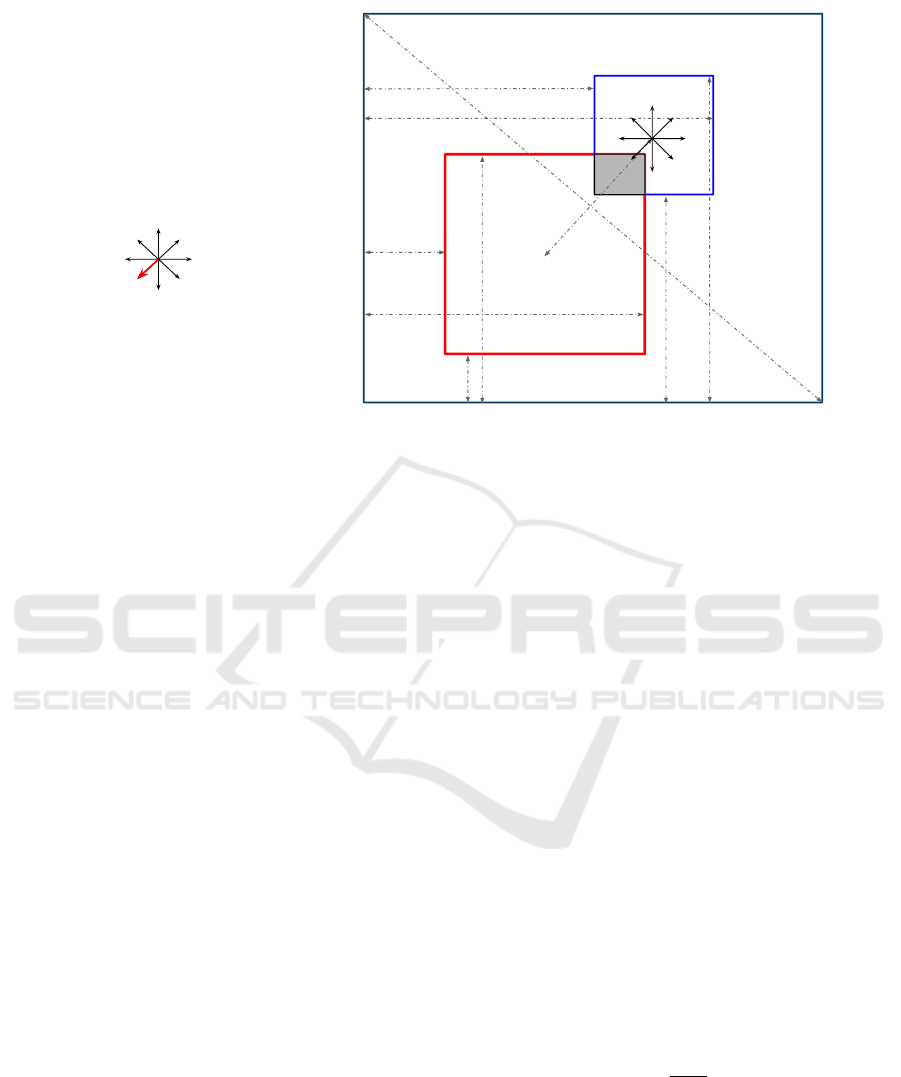
F
2
= A
o
/ A
I
F
3
= A
1
/ A
I
F
4
= A
0
/ A
1
F
5
= d
obj
/ d
i
F
6
= Area(OVLP) / smallest(A
0
, A
1
)
F
7
= d
obj
/ 0.5 [(A
0
+A
1
)]
0.5
F
8
=
F
9,11
= (a
1
- a
0
) / (b
0
- a
0
)
F
10,12
= (b
1
- a
0
) / (b
0
- a
0
)
F
13, 14
= w / h
d
i
＋
obj
0
＋
obj
1
OVLP
I
A
0
= Area(obj
0
)
A
1
= Area(obj
1
)
A
I
= Area(I)
d
obj
a
0
b
0
a
1
b
1
a
0
b
0
a
1
b
1
w
w
h
h
Figure 2: Geometric features proposed by Muscat and Belz (2017).
a
0
). Similarly, F
11
and F
12
are computed with re-
spect to the image’s bottom edge and the bound-
ing boxes’ horizontal edges respectively.
• F
{13,14}
: Aspect ratio of the width to height of
each bounding box.
Depth Features (DF): To also consider the z-
dimension of each object, human estimated depths
were also included as part of the visual feature set.
Depth estimates were collected in (Birmingham et al.,
2018) after instructing annotators to specify their esti-
mated average depth in the range between 0 and 100.
In this study, depth values for the two objects were
normalised between 0 and 1 {F
d
| 15 ≤ d ≤ 16}
and depth difference F
17
between ob j
0
and ob j
1
was
computed to reflect the depth order of the two objects.
4 METHODOLOGY
To build a multi-label machine-learning model while
simultaneously projecting the relationship between
the various spatial relations, an unsupervised cluster-
ing approach was developed. The approach is de-
signed to group similarly oriented spatial relations
based on their linguistic and visual properties. By
making use of the k-means clustering algorithm (Pe-
dregosa et al., 2011) and without taking into consider-
ation the ground-truth preposition sets, the scaled fea-
ture vectors having zero mean and unit variance were
grouped into k distinct clusters. The probability distri-
bution of prepositions across each cluster and thresh-
olded at t was exploited for both the classification of
unseen instances as well as for preposition similarity.
4.1 Model
The developed model is based on k-means clus-
tering which aims to partition the instance space
X into k disjointed and non-hierarchical clusters
and represented by set C (Jain et al., 1999). The
method is designed to iteratively assign each x
i
∈ X
into one of the available clusters defined in set
C in a 2-stepped approach until a terminating
condition is met. Starting from an initial set of k
centroids represented by the randomly initialised
means M
(t)
= {m
(t)
1
,m
(t)
2
,. .. ,m
(t)
k
} at time-step t,
each having a dimension |x
i
|, the first step requires
the assignment of each instance x
i
to the closest
cluster centroid based on Euclidean distance. This is
calculated between x
i
∈ X and m
i
∈ M, such that each
cluster c
(t)
∈ {C
(t)
c
|1 ≤ c ≤ k} is composed of:
{x
i
: ||x
i
− m
(t)
c
||
2
≤ ||x
i
− m
(t)
j
||
2
∀
j
,1 ≤ j ≤ k},
where each x
i
is assigned to only one cluster c
(t)
irrespective of any instances which might fit in mul-
tiple clusters. The algorithm continues by updating
each cluster mean found in set M by:
m
(t+1)
c
=
1
|c
(t)
|
∑
x
i
∈c
(t)
x
i
. (1)
These two steps are repeated until either the cen-
troids and instances stabilise (i.e., centroids stop
changing their position and instances keep consistent
cluster membership), or until a number of iterations
are performed. Given the non-deterministic nature of
this method and since it does not guarantee a global
ICINCO 2019 - 16th International Conference on Informatics in Control, Automation and Robotics
150

optimum, initial centroid seeds are initialised via the
k-means++ algorithm (Arthur and Vassilvitskii, 2007)
to speed up convergence. Furthermore, the method
was executed for 1000 consecutive runs and each run
was allowed to perform 300 iterations. This was per-
formed to increase the likelihood of finding the cen-
troids that best minimise the within-cluster variance.
Once the set of data points X are clustered in the
final number of k clusters, multi spatial relation detec-
tion is implemented by first computing the preposition
likelihoods P(P |C) for each spatial preposition p
i
∈ P
over each cluster c
i
∈ C. Preposition likelihoods are
then normalised with respect to the maximum likeli-
hood found per each cluster c
i
, such that the dominant
prepositions found within each cluster have a likeli-
hood equal to 1 given that:
P(p
i
|c
j
) =
P(p
i
|c
j
)
argmax
p
i
P(p
i
|c
j
)
. (2)
4.2 Classification
The multi spatial relation set for a given unseen object
pair represented by x
i
is predicted by a two-stepped
approach. The first step is to find the closest cluster
C
m
represented by its mean m that minimises the L
2
norm distance among all cluster means by:
m = argmin
m∈M
{||x
i
− m||
2
}. (3)
The second step is to extract the prepositions be-
longing to the closest cluster C
m
which have a likeli-
hood ratio that exceeds a specified threshold t. Math-
ematically, the predicted spatial relations h(x
i
) are de-
noted by:
h(x
i
) = {p
i
: P(p
i
|C
m
) ≥ t}. (4)
The training phase and the details for optimising
the hyper-parameters k and t of the presented model
are discussed in subsection 4.5.
4.3 Distance Metric
To get deeper insights into how prepositions are re-
lated to each other, the clustering-based model offers
a way to compute the similarity between each prepo-
sition p
i
∈ P. By representing how each preposition p
i
is clustered through its distribution over each cluster
c
i
∈ C, spatial prepositions can be compared via a dis-
tribution distance metric. Given that the prepositions
p
{i, j}
are represented by the probability distributions
P(C | p
{i, j}
), prepositions were compared via the his-
togram intersection method which computes the dis-
tance metric d(p
i
, p
j
) as follows:
d(p
i
, p
j
) =
∑
c
k
∈C
min(P(c
k
| p
i
), P(c
k
|p
j
)) (5)
4.4 Evaluation Metrics
Hyper-parameter optimisation and evaluation were
both performed after splitting the dataset into devel-
opment (80%) and test set (20%). The development
set was further sub-divided into training and valida-
tion sets in the same ratio for hyper-parameter optimi-
sation purposes. The developed model h(·) was opti-
mised by minimising the difference between the full
dataset’s (D) overall label cardinality (i.e., the aver-
age number of labels per instance which is equal to
2.16), and the average predicted preposition set size
for the test set. The label cardinality (LCard) for
dataset D is computed by:
LCard(D) =
1
m
m
∑
i=1
|Y
i
|, (6)
where m is the total number of instances in the
pertaining set.
Example-based metrics, accuracy (Acc), precision
(P), recall (R) and F-score (F), were used to evaluate
the multi-label classifier. These metrics were com-
puted between the ground-truth labels Y and the pre-
dicted spatial preposition sets
ˆ
Y = {h(x
i
), ∀
x
i
∈ X},
over each test instance computed by:
Acc =
1
m
m
∑
i=1
|Y
i
∩ h(x
i
)|
|Y
i
∪ h(x
i
)|
; (7)
P =
1
m
m
∑
i=1
|Y
i
∩ h(x
i
)|
|h(x
i
)|
; (8)
R =
1
m
m
∑
i=1
|Y
i
∩ h(x
i
)|
|Y
i
|
; (9)
F =
1
m
m
∑
i=1

2 × P
i
× R
i
P
i
+ R
i

, (10)
where m is the number of test instances, Y
i
is the
ground-truth spatial relation set for the i
th
instance,
x
i
is the i
th
feature vector, and h(x
i
) is the predicted
spatial relation set for x
i
by the classifier h(·).
4.5 Optimisation
The above metrics were computed under various k
and t values to gain insight into how the clustering-
based model performs under both linguistic and visual
features. The first experiment was carried out to eval-
uate the model based solely on linguistic properties.
This was intended to identify the language feature set
Clustering-based Model for Predicting Multi-spatial Relations in Images
151

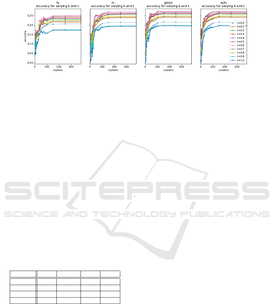
Figure 3: Accuracies computed on the validation set for varying clusters (k) and thresholds (t) based on linguistic features
including Label Encoding (LE), Indicator Vector (IV), GloVe and Word2Vec (W2V) word embeddings.
that best represents the object labels whilst also max-
imising the discussed evaluation metrics. Figure 3,
shows the accuracies obtained when predicting spa-
tial relations for the instances found in the validation
set based on each linguistic feature set. The plots
show how the accuracy varies with the different num-
ber of clusters (k) and thresholds (t). The accuracy
peaks when approaching the 100
th
cluster for all var-
ied thresholds, and the top two performing thresholds
where 0.5 and 0.6 for each configuration. Further-
more, it is evident that the Indicator Vector (IV) fea-
ture set marginally improves on the Label Encoding
(LE), while the GloVe and Word2Vec (W2V) slightly
outperform the IV. When analysing the overall accu-
racies for each feature set computed across all k and t
values (i.e., total of 342 per each feature set), Table 2
shows that the highest accuracy recorded is 0.273 for
both GloVe and W2V embeddings, while the highest
accuracy mean (0.195) and median (0.198) were ob-
tained when using GloVe features. For this reason, the
GloVe feature set was used for the following experi-
ments in conjunction with both geometric and depth
features.
Table 2: Overall statistics per each linguistic feature set.
Features Mean Median Min Max
LE 0.172 0.166 0.042 0.250
IV 0.180 0.180 0.132 0.270
W2V 0.187 0.196 0.153 0.273
GloVe 0.195 0.198 0.164 0.273
The hyper-parameters k and t were both optimised
with respect to the corresponding average predicted
preposition set size as obtained on the validation set.
As shown in Figure 4, the model was assessed in
terms of how many prepositions are generated for a
given unseen instance when represented by a combi-
nation of linguistic and visual features. This was per-
formed for varying values of k and t. The plots show
that when the model is parameterised with thresholds
of 0.5 and 0.6, it gives an average preposition set size
that is very comparable to the overall dataset’s label
cardinality (i.e., 2.16 and which is marked by the hor-
izontal dashed line in the respective plots), given that
the number of clusters (k) falls within the stable re-
gion (i.e., within the elbow curve which is represented
by the vertical dashed line in the plots). Therefore,
the number of optimal clusters for each configuration
is set to 150, while a threshold t = 0.6 is used when
the model is based on: {GloVe, GF, GloVe+GF} sets,
and t = 0.5 is set when the model uses the combined
feature set composed of: {Glove+GF+DF}.
The remaining evaluation metrics associated with
the respective chosen hyper-parameters are tabulated
in Table 3. The table shows that the linguistic fea-
tures highly influence the spatial relation detection.
The accuracy obtained based only on linguistic fea-
tures is 0.273. The accuracy decreased to 0.211 when
spatial relations were predicted based on their geo-
metric features. When both feature sets were com-
bined (i.e, GloVe+GF), the average precision (AP)
increased by 3.1%, over that obtained when using
GloVe features alone, while the average recall (AR)
decreased by 8.3% which resulted in a loss of 1.1%
in accuracy. However, when adding the depth features
together with the linguistic and geometric properties
(i.e., GloVe+GF+DF), the average accuracy (Acc) in-
creased by 3.7% and reached the highest recorded ac-
curacy of 0.283, thus confirming the effectiveness of
the added depth features.
5 RESULTS AND DISCUSSION
The final models were trained on the full develop-
ment set with k = 150 for all feature sets. The likeli-
hood threshold t was set to 0.5 when the models were
trained on the complete feature set, while for the other
cases, t was set to 0.6. Each trained model was evalu-
ated on the testing set for 50 times to compute the av-
erage metrics which are reported in Table 4. This was
also intended to calculate the average recall per spa-
tial relation as can be found in Table 5. The latter re-
ICINCO 2019 - 16th International Conference on Informatics in Control, Automation and Robotics
152

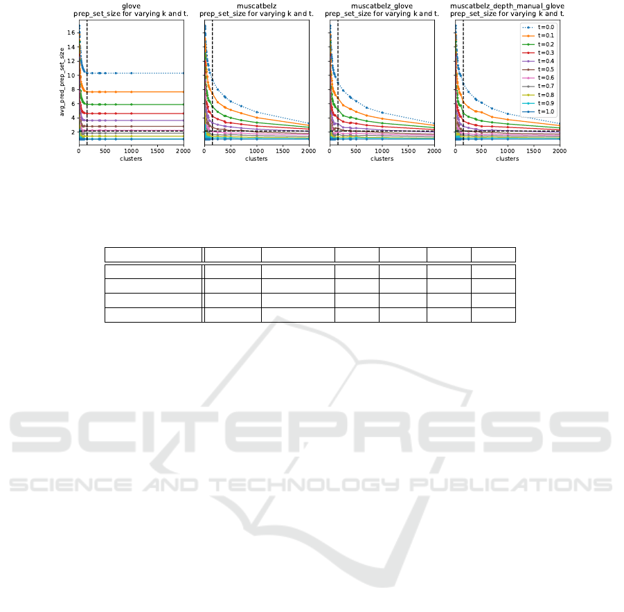
Figure 4: Average predicted preposition set sizes generated for the validation set for varying clusters (k) and thresholds (t)
based on a combination of linguistic and visual features. The plots show the dataset’s average prepositions set size (i.e., 2.16)
and the region where cluster stabalise (i.e., @k = 150) with the horizontal and vertical dashed lines respectively.
Table 3: Evaluation metrics computed on the validation set for each feature vector.
Features k,t LCard(Val) Acc P R F
GloVe 150, 0.6 2.265 0.273 0.356 0.385 0.343
GF 150, 0.6 2.079 0.211 0.276 0.307 0.269
GloVe+GF 150, 0.6 2.004 0.270 0.367 0.353 0.336
GloVe+GF+DF 150, 0.5 2.167 0.283 0.370 0.388 0.353
sults were compared to those obtained by the best per-
forming single-label classifier (i.e., Random Forest),
as reported by Muscat and Belz (2017). Furthermore,
the similarity measure between each preposition was
calculated based on the best performing multi-label
model and is presented by Figure 5.
Table 4 confirms the importance of the linguistic
features when predicting spatial relations. The aver-
age accuracy rate (A-Acc) when using only linguistic
features is equal to 0.271. The accuracy decreased to
0.229 when considering only the geometric orienta-
tion setup between the image objects. Although by
using both linguistic and geometric feaures, the aver-
age precision (AP) increased by 3.8% over that ob-
tained when using GloVe features alone, the average
recall (AR) decreased from 0.391 to 0.335. This re-
sulted in an accuracy of 0.260 which implies a de-
crease of 4.1%. The introduction of the depth features
(DF) resulted in the achievement of the highest eval-
uation metrics. Specifically, the accuracy increased
by a margin of 9.6% and hence resulted in an overall
accuracy of 0.285.
Table 5 shows the average recall per spatial rela-
tion (SR) for all feature sets along with the recall@k
obtained by the top performing single label classifier
that was reported by Muscat and Belz (2017). The
per-preposition recall results were combined with the
number of training and testing instances which were
used for each model. The benefit of the linguistic
features (LF) was most notably seen when predict-
ing the spatial relations: along, around, on, outside
of, and under, after exceeding the 0.7 average recall
mark. Despite reducing the average recall (AR) from
0.391 to 0.333, the geometric features (GF) alone im-
proved six out of all the total (17) relations which in-
cluded: beyond, far from, in, in front of, none, and
opposite. This confirmed that the latter set of rela-
tions were more distinguishable based on their geo-
metric setup rather than the inherent language bias of
the corresponding image objects. When combining
both LF and GF, the AP was increased to 0.335 but
this was still not better than the 0.391 mark which was
recorded by the LF. Despite this outcome, the average
recalls for the latter set of prepositions together with 3
additional relations (total of 9), including behind, on,
and under were improved over the results obtained by
the LF. After adding the depth features (DF), the lat-
ter set of spatial relations improved even more, except
the preposition on which kept the same recall rate (re-
duced from 0.83 to 0.82). The most notable percent-
age gains were noted for the prepositions in front of
(66.7%), far from (60.9%), behind (46.1%), and be-
yond (45%).
We also trained a Random Forest single label clas-
sifier which gave best results in (Muscat and Belz,
2017) to show the effectiveness of the designed ap-
proach. The single label classifier was trained on the
full feature set and optimised by hyperparamer opti-
misation. The model is based on 10 estimators and
has a maximum depth of 5 levels. The maximum ac-
curacy obtained on the validation set based on the op-
timal hyperparameters was 0.35, while the accuracy
on the testing set was to 0.34. This final model was
trained on the development set for 50 times to evalu-
ate the average recall@k per each preposition.
Table 5 (right side) gives the average per-
preposition recall@k, k=1..4, although in practice the
recall@1 is used for single-label prediction cases.
Clustering-based Model for Predicting Multi-spatial Relations in Images
153

Table 4: Average metrics computed over 50 runs on the testing set for each feature set.
Features k,t A-LCard(Test) A-Acc AP AR AF
GloVe 150, 0.6 2.375 0.271 0.338 0.391 0.337
GF 150, 0.6 2.305 0.229 0.292 0.333 0.291
GloVe+GF 150, 0.6 2.000 0.260 0.351 0.335 0.320
GloVe+GF+DF 150, 0.5 2.335 0.285 0.365 0.400 0.354
Table 5: Average recall per spatial relation (SR) computed over 50 times on the testing set. Each preposition is combined
with the corresponding number of instances which were used during training and testing. Average recalls obtained by GF are
compared to the Recall@k obtained by the best performing single label classifier (i.e., Random Forest) as reported by Muscat
and Belz (2017) when trained on the full feature set.
Multi-label Model Random Forest Classifier
Average Recall Recall@k
French SR
(English SR)
Training
instances
Testing
instances
GloVe GF GloVe+GF GloVe+GF+DF k=1 k=2 k=3 k=4
au dessus de
(above)
102 22 0.43 0.30 0.41 0.44 0.00 0.00 0.00 0.05
contre
(against)
463 150 0.39 0.32 0.25 0.27 0.01 0.53 0.64 0.79
le long de
(along)
54 19 0.82 0.35 0.75 0.81 0.00 0.00 0.00 0.00
autour de
(around)
28 7 1.00 0.89 0.90 1.00 0.15 0.24 0.32 0.48
au dessus de
(at the level of )
745 246 0.64 0.56 0.58 0.59 0.00 0.00 0.68 0.84
derri
`
ere
(behind)
846 279 0.09 0.07 0.13 0.19 0.38 0.70 0.80 0.87
par del
`
a
(beyond)
33 5 0.11 0.33 0.20 0.29 0.00 0.00 0.01 0.11
loin de
(far from)
300 104 0.17 0.28 0.23 0.37 0.01 0.66 0.84 0.91
dans
(in)
43 18 0.60 0.64 0.63 0.69 0.04 0.05 0.09 0.16
devant
(in front of )
863 260 0.11 0.19 0.12 0.20 0.42 0.62 0.73 0.86
pr
`
es de
(near)
1820 573 0.41 0.22 0.19 0.30 0.78 0.95 1.00 1.00
`
a c
ˆ
ot
´
e de
(next to)
1159 328 0.51 0.47 0.43 0.49 0.00 0.62 0.91 0.97
aucun
(none)
16 6 0.17 0.20 0.25 0.34 0.00 0.00 0.00 0.00
sur
(on)
296 87 0.76 0.69 0.83 0.82 0.67 0.72 0.77 0.81
en face de
(opposite)
207 70 0.35 0.41 0.40 0.39 0.00 0.01 0.05 0.11
`
a l’exterieur de
(outside of )
28 13 0.88 0.38 0.79 0.84 0.00 0.00 0.00 0.00
sous
(under)
341 109 0.72 0.62 0.74 0.75 0.61 0.64 0.67 0.75
Mean Average Recall 0.48 0.41 0.46 0.52 0.18 0.34 0.44 0.51
From these results (recall@1), we see that the multi-
label model improved the recall for 14 out of 17
prepositions (including the aucun (“none”) option)
and obtained lower recall rates for the three preposi-
tions: devant (“in front of”), derri
`
ere (“behind”) and
pr
`
es de (“near”). When taking into account that the
dataset’s cardinality was 2.16, the multi-label model
still improved 11 prepositions when considering the
recall@2 obtained by the Random Forest. The mean
average recall for the multi-label model was equal to
0.52, whilst the mean average recall@1 that was ob-
tained by the single label classifier was 0.18. The sin-
gle label classifier obtained comparable rate at k = 4
since it predicted prepositions with a recall rate of
0.51. When taking into consideration the results
achieved by the single label classifer @k = 4, it still
underperformed in 10 prepositions while it obtained
equal rate for the preposition under. This confirmed
ICINCO 2019 - 16th International Conference on Informatics in Control, Automation and Robotics
154

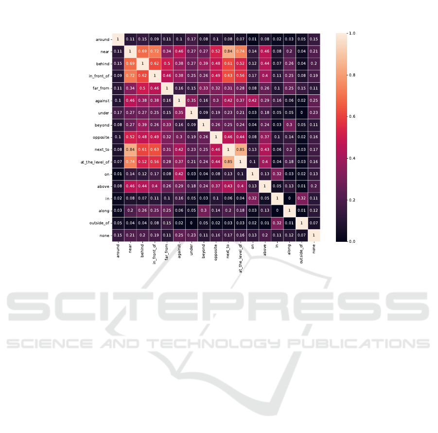
Figure 5: Similarity between prepositions based on the their clustering distribution.
that the multi-label model is generally performing
better than the single label classifier even when con-
sidering recall rates with k greater than the dataset’s
label cardinality.
Figure 5 presents how prepositions are related in
terms of how similar they are to each other based on
their clustering distribution. The plot shows that the
prepositions near and next to share common charac-
teristics with other relations. Specifically, the spatial
relation near is similar to next to (0.84), at the level
of (0.74), in front of (0.72), and behind (0.69). Sim-
ilarly, the preposition next to is similar to at the level
of (0.85), near (0.84), in front of (0.63), and behind
(0.61).
6 CONCLUSION AND FUTURE
WORK
In this paper we reported on the development of a
clustering-based model which we used to study the re-
lations between prepositions and to generate a multi-
label output. The analysis of the clusters shows that
the prepositions near, next to and at the level of have
similar feature characteristics and it may be difficult
to model their fine-grained distinctions. We evaluated
the performance of the multi-label prediction model,
which takes as input linguistic, geometric and depth
features and a comparison with a single-label Ran-
dom Forest model shows that the majority of preposi-
tions benefit from the multi-label model. In the near
future, we will explore other clustering-based algo-
rithms used in multi-label classification, and imple-
ment a multi-label Neural Network model, which can
help us study the features that distinguish the applica-
tion of each preposition in more depth.
REFERENCES
Arthur, D. and Vassilvitskii, S. (2007). K-means++: The
advantages of careful seeding. In Proceedings of
the Eighteenth Annual ACM-SIAM Symposium on
Discrete Algorithms, SODA ’07, pages 1027–1035,
Philadelphia, PA, USA. Society for Industrial and Ap-
plied Mathematics.
Belz, A., Muscat, A., Aberton, M., and Benjelloun, S.
(2015). Describing spatial relationships between ob-
jects in images in english and french. In 4th Workshop
on Vision and Language, pages 104–113, Lisbon, Por-
tugal.
Belz, A., Muscat, A., Anguill, P., Sow, M., Vincent, G.,
and Zinessabah, Y. (2018). Spatialvoc2k: A multilin-
gual dataset of images with annotations and features
for spatial relations between objects. In Proceedings
of the 11th International Conference on Natural Lan-
guage Generation.
Clustering-based Model for Predicting Multi-spatial Relations in Images
155

Birmingham, B., Muscat, A., and Belz, A. (2018). Adding
the third dimension to spatial relation detection in 2d
images. In Proceedings of the 11th International Con-
ference on Natural Language Generation, pages 146–
151.
Carlson-Radvansky, L. A. and Logan, G. D. (1997). The
influence of reference frame selection on spatial tem-
plate construction. JOURNAL OF MEMORY AND
LANGUAGE, 37:411–437.
Carlson-Radvansky, L. A. and Radvansky, G. A. (1996).
The influence of functional relations on spatial term
selection. Psychological Science, 7(1):56–60.
Coventry, K. R., Prat-Sala, M., and Richards, L. (2001). The
interplay between geometry and function in the com-
prehension of over, under, above, and below. Journal
of Memory and Language, 44(3):376 – 398.
Dai, B., Zhang, Y., and Lin, D. (2017). Detecting visual
relationships with deep relational networks. In Com-
puter Vision and Pattern Recognition (CVPR), 2017
IEEE Conference on, pages 3298–3308. IEEE.
Dobnik, S. and Kelleher, J. (2014). Exploration of func-
tional semantics of prepositions from corpora of de-
scriptions of visual scenes. In Proceedings of the
Third Workshop on Vision and Language, pages 33–
37. Dublin City University and the Association for
Computational Linguistics.
Jain, A. K., Murty, M. N., and Flynn, P. J. (1999). Data
clustering: a review. ACM computing surveys (CSUR),
31(3):264–323.
Kelleher, J. D. and Kruijff, G.-J. (2005). A context-
dependent algorithm for generating locative expres-
sions in physically situated environments. In Proceed-
ings of the Tenth European Workshop on Natural Lan-
guage Generation (ENLG-05).
Kelleher, J. D., Ross, R. J., Sloan, C., and Namee, B. M.
(2011). The effect of occlusion on the semantics of
projective spatial terms: a case study in grounding lan-
guage in perception. Cognitive Processing, 12(1):95–
108.
Logan, G. D. and Sadler, D. D. (1996). A computa-
tional analysis of the apprehension of spatial rela-
tions, pages 493–529. The MIT Press, Cambridge,
MA, US.
Lu, C., Krishna, R., Bernstein, M., and Fei-Fei, L. (2016).
Visual relationship detection with language priors.
In European Conference on Computer Vision, pages
852–869. Springer.
Mikolov, T., Sutskever, I., Chen, K., Corrado, G. S., and
Dean, J. (2013). Distributed representations of words
and phrases and their compositionality. In Advances in
neural information processing systems, pages 3111–
3119.
Muscat, A. and Belz, A. (2017). Learning to generate
descriptions of visual data anchored in spatial rela-
tions. IEEE Computational Intelligence Magazine,
12(3):29–42.
Pedregosa, F., Varoquaux, G., Gramfort, A., Michel, V.,
Thirion, B., Grisel, O., Blondel, M., Prettenhofer,
P., Weiss, R., Dubourg, V., Vanderplas, J., Passos,
A., Cournapeau, D., Brucher, M., Perrot, M., and
Duchesnay,
´
E. (2011). Scikit-learn: Machine learning
in Python. Journal of Machine Learning Research,
12:2825–2830.
Pennington, J., Socher, R., and Manning, C. (2014). Glove:
Global vectors for word representation. In Proceed-
ings of the 2014 conference on empirical methods in
natural language processing (EMNLP), pages 1532–
1543.
Ramisa, A., Wang, J., Lu, Y., Dellandrea, E., Moreno-
Noguer, F., and Gaizauskas, R. (2015). Combining
geometric, textual and visual features for predicting
prepositions in image descriptions. In Proc. 20th
Conf. on Empirical Methods in Natural Language
Processing (EMNLP), pages 214–220, Lisbon, Portu-
gal.
Regier, T. and Carlson, L. A. (2001). Grounding spatial
language in perception: an empirical and computa-
tional investigation. Journal of Experimental Psychol-
ogy General, 130(2):273–298.
Sadeghi, M. A. and Farhadi, A. (2011). Recognition us-
ing visual phrases. In Computer Vision and Pat-
tern Recognition (CVPR), 2011 IEEE Conference on,
pages 1745–1752. IEEE.
Tsoumakas, G. and Katakis, I. (2007). Multi-label classi-
fication: An overview. Int J Data Warehousing and
Mining, 2007:1–13.
Yu, R., Li, A., Morariu, V. I., and Davis, L. S. (2017). Visual
relationship detection with internal and external lin-
guistic knowledge distillation. In IEEE International
Conference on Computer Vision (ICCV).
Zhang, M. and Zhou, Z. (2014). A review on multi-label
learning algorithms. IEEE Transactions on Knowl-
edge and Data Engineering, 26(8):1819–1837.
ICINCO 2019 - 16th International Conference on Informatics in Control, Automation and Robotics
156