Research on Rail Potential While Many Trains Are Starting at the

Same Time

Jie Hao

1, a

, Chuyan Xi

2, b

, Xinyuan Liu

1, c

, Huiping Zheng

1, d

, Ying Qu

1, e

and Yifan Zhang

1, f

State Grid Shanxi Electric Power Research Institute; QingNian rd. no.6;Taiyuan;China

State Grid Taiyuan Power Supply Company; BingZhou North Rd. NO. 89;Taiyuan;China

quying20090244@163.com,

358465506@qq.com

Keywords: Traction current; many trains; start; rail potential.

Abstract: The value of traction current affects rail potential. In real life, if many trains start at the same time, the traction

current may increase, and so is the rail potential. The excessive rail potential would seriously threaten people’s

lives. The paper states briefly that many trains start at the same time will increase the traction current and the

rail potential, and it is verified by the Matlab/simulink model and the field test data. Lastly, an optimization

measure of traction current based on locomotive schedule is proposed to reduce the rain potential.

1 UNTRODUCTION

The rapid development of urban rail transit brings a

lot of convenience to people. However, some new

problems such as stray current corrosion and high

orbital potential were on the way. Once the rail

potential is too high, people will have electric shock

hazard. Therefore, the reason of studying orbital

potential, which proposes the inhibitory measures of

orbital potential is particularly important.

Research shows the magnitude of locomotive

traction current can affects the height of orbital

potential. With larger locomotive traction current

comes higher orbital potential (YANG Gang, 2010).

In real life, different execution mode of locomotives

can affects the size of traction current. When the train

is in an accelerated stated, absorbing current from the

power grid. When multiple columns of locomotive

starts at the same time, also causes the increase of

traction current (WANG Jia, 2012).

2 UNDER CERTAIN CONDITION

OF MULTIPLE LOCOMOTIVES

START AT THE SAME TIME,

THEORETICAL

CALCULATION AND

ANALYSIS OF TOTAL

TRACTION CURRENT SIZE

Regard the time of the first locomotive left the

departure station as zero hour, set the traction current

which comes from the locomotive’s parking time at

each station are all zero seconds to i(t,0), where t is

the running time. According to the actual situation,

the duration of the locomotive’s stay at each station

can be adjusted (LI Guoxin, 2010). Assume the time

range of the locomotive’s adjustable action at the

No.m station is [a

, b

] seconds, the traction current

for the first vehicle at this time can be expressed as

(, ) (, )

tT itT

(1)

In this formula,

1111

[ , ,... ]

Tttt

is the vector of

the residence time of the first vehicle at each station.

N is the total number of stations,I (t,T

) is a function

about time and locomotive traction current based I

(t,0) on and T

. The Fixed D-value to i(t,0) can be

made in accordance with the parking time per station

at the time of the specific calculation. (Because the

Hao, J., Xi, C., Liu, X., Zheng, H., Qu, Y. and Zhang, Y.

Research on Rail Potential While Many Trains Are Starting at the Same Time.

DOI: 10.5220/0010009400170021

In Proceedings of the International Symposium on Frontiers of Intelligent Transpor t System (FITS 2020), pages 17-21

ISBN: 978-989-758-465-7

locomotive lighting, signal, door and other systems

are still in working condition when parking, the

traction current is not zero).

Set the departure interval to n seconds, the

traction current of the P vehicle can be expressed as

(, ) ( , )

tT it pnT

(2)

Set the maximum number of locomotives running

at the same time on the running route is P, these steps

allow you to get the total current value of the whole

line at any time.

(, ) (, )

tT f tT





(3)

As the locomotive quickened its advance, it

absorbs electricity from the grid. Therefore,

(, ) 0

ftT 

. According to formula (3), when there

are multiple locomotives increase the speed of start-

up at the same time on the line, the total traction

current will be increased (M. Brenna, A. Dolara,S.

Leva, D, 2010).

3 MATLAB/SIMULINK

SIMULATION ANALYSIS AND

FIELD RECORD DATA

WAVEFORM VERIFICATION

This article selects the “Rail-Exhaust network-

Groung-Buried metal” model that is closest to the

actual. Separately in One-way Feeding style and

Two-way Feeding style, making simulation analysis

to the model, used to study the effects to rail potential

under a certain state when multiple locomotives

increase the speed of start-up at the same time.

(1) “Rail-Exhaust network-Groung-Buried

metal” equivalent circuit when in the One-way

Feeding style as shown in the figure 1:



机车1 机车2

钢轨

排流网

大地

埋地金

属

Rpd

Rdm

Rgp



‐

Figure 1: Equivalent circuit under unilateral power supply.

Combining with the actual situation, setting

simulation parameters: Set the 3 substation spacing to

a power supply range, then establish a power supply

range.

Take part of the parameter to a specific value:

DC=750V, Rail longitudinal resistance=0.03

km

Earth longitudinal resistance=0.001

km

, Exhaust

network=0.001





, Buried metal longitudinal

resistance=0.005





, Transition resistance

between track and exhaust network=15

km

Transition resistance between the exhaust network

and the earth=3





, Transition resistance between

the earth and buried metal=3

km

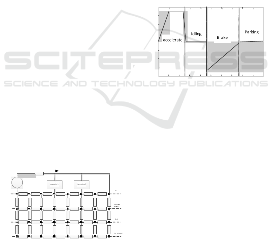
Replace the the locomotive with the controlled

current source, refer to relevant information (M.

Brenna, A. Dolara,S. Leva, D, 2010), set the absorbed

current curve during locomotive operation, as shown

in the figure 2:

015105203530

504540

-800

-600

-400

-200

200

400

600

800

加速惰行刹车

停车

t/s

I/A

Figure 2: Diagram of the absorbed current by locomotive

during running.

Because this paper mainly studies the influence of

track potential when locomotive speed up startup,

choose a simulation time of 0 to 25 seconds, to ensure

that locomotives operate faster during this time

period.

Regard the position of the substation is 0(

0kmL



). Locomotives begin to accelerate from

0kmL



at zero of the relative time, the locomotive

starts to accelerate at a

1.2kmL  seconds later,

mapping within the same coordinate system. When

two locomotives are individually accelerated and

simultaneously accelerated, a curve in which the

orbital potential changes over time at a certain point

0.6kmL



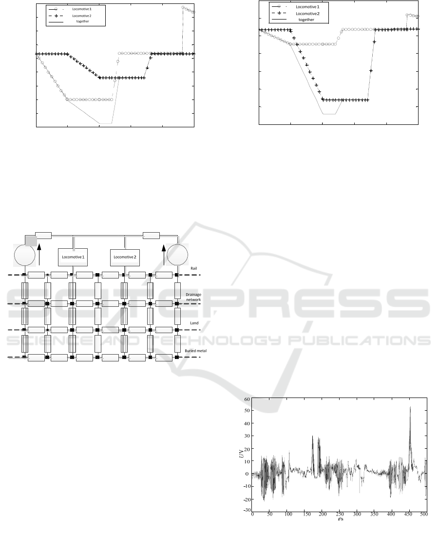
in the interval as shown in the

following figure 3:

FITS 2020 - International Symposium on Frontiers of Intelligent Transport System

??1????

??2????

???????

10 15 20

-144

-143

-142

-141

-140

-139

-138

-137

-136

-135

t/s

U/V

Figure 3: Diagram of the rail potential located at

0.6kmL 

changing by time when two locomotives

accelerate separately and simultaneously.

(2) Equivalent circuits in “Rail-Exhaust network-

Groung-Buried metal” model under bilateral are

shown in the figure 4:



机车1

钢轨

排流网

大地

DC1

Rpd

Rdm

Rgp



DC2

埋地金

属

机车2

‐

Figure 4: Equivalent circuit under bilateral power supply.

Parameter settings are the same as parameter

settings under unilateral power supply mode.

Set the location of substation 1 is

0kmL  . The

first vehicle speed up from

0kmL  at the moment

of relative time, the locomotive starts to accelerate at

3.6kmL  in 25 seconds. Mapping within the same

coordinate system, when two locomotives are

individually accelerated and simultaneously

accelerated during operation, the change curve of

orbital potential at a certain point of

1.8kmL  in the

interval is shown in the figure 5 respectively:

??1????

??2????

???????

10 15 20 25

t/s

-240

-230

-220

-210

-200

-190

-180

-170

U/V

Figure 5: Diagram of the rail potential located at

1.8kmL



changing by time when two locomotives

accelerate separately and simultaneously.

Comparing the above modes of power supply, it

can be seen from the waveform diagram of the

influence of locomotive startup acceleration

operation on rail potential, when two locomotives

accelerate operation at the same time, relative to the

case of each locomotive running alone, the orbital

potential will all increase, there’s just a difference in

a value. Therefore we can conclude that the

simultaneous start of the train will cause the traction

current to increase, which causes an increase in

orbital potential.

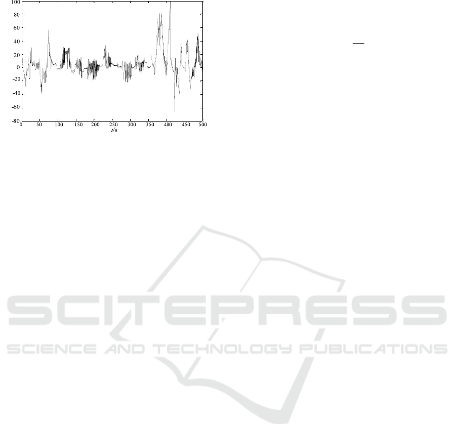
The following is a waveform based on the

measured data in the field. In both cases, when a

locomotive starts to accelerate operation and multiple

locomotive start to accelerate operation at the same

time, the curve of orbital potential changing with time

at a certain point along the route is shown in the figure

6 and 7:

Figure 6: Diagram of the rail potential located at a point

changing by time when one locomotive accelerate.

Research on Rail Potential While Many Trains Are Starting at the Same Time

U/V

Figure 7: Diagram of the rail potential located at a point

changing by time when several locomotive accelerate.

Comparing figures 6 and 7, we can see that the

orbital potential increases when multiple locomotives

accelerate operation at the same time, as opposed to a

single locomotive starting the accelerated operation

alone.

Therefore, in order to reduce the orbital potential,

we can adjust the locomotive scheduling time,

reducing the probability of simultaneous start-up

operation of multiple locomotives, making some

optimization of the traction current.

4 OPTIMIZATION OF

TRACTION CURRENT BASED

ON LOCOMOTIVE

DISPATCHING

When the locomotive is running, the residence time

of the locomotive at each station can be adjusted

according to the allowable range. Therefore, the time

of station stay along the route can be reasonably

optimized to reduce the simultaneous start-up

operation probability of multiple locomotives.

According to the above ideas, traction current

optimization based on locomotive dispatching can be

realized by the following two methods:

1) Calculate the total value and take the minimum.

For each set of locomotives can be achieved at each

station residence time, Calculating the corresponding

scheduling schedule separately, and using it as the

final scheduling schedule. Due to the long running

time of the locomotive throughout the day, the

calculation of this method is too heavy, so it’s not

feasible.

2) Establishing the mathematical model of using

locomotive residence time to reduce total traction

current, solving the minimum values. At the same

time, up to



(4)

Locomotives were running at the same time, in

the above formula, M is the maximum time allowed

for a locomotive from the point of departure to the

end, and N is the fixed departure interval for

locomotive dispatching. Also, from the beginning of

the P-1 vehicle, a loop is formed at the NP time

interval, so it is calculated only within the [N (P-1), N

(P-1) +NP] time frame. Make the running schedule of

the P vehicle, and the subsequent locomotives

recycling uses this schedules.

The impact model used to reduce the total traction

current by adjusting the residence time of each station

can be expressed as:

min max{ ( , )}

(5)

.. ( 1) (2 1)st n P t n P



≤≤

(6)

mm m

atb≤≤

(7)







(8)

In formula (8), C is the maximum allowable time

for stays along the locomotive, which is a nonlinear

and extremely small problem. By calculation, the

value of the minimum traction current can be solved.

5 CONCLUSION

Based on the actual situation, this paper establishes a

“Rail-Exhaust network-Groung-Buried metal” four-

layer model, and under the two power supply modes

of unilateral power supply and bilateral power supply,

the model is simulated and verified by the actual test

data, and the results show that the rail potential is

increased by the simultaneous start-up operation of

multiple locomotives. By establishing the

mathematical model of locomotive residence time to

reduce the total traction current, it is a measure to

reduce the rail potential by reasonably optimizing the

station residence time along the locomotive.

FITS 2020 - International Symposium on Frontiers of Intelligent Transport System

REFERENCES

LI Guoxin. Analysis of DC Traction Reflux System and

Research on Related Problems in Rail Potential. China

University of Mining and Technology Doctor Degree

Thesis,2010.

M. Brenna, A. Dolara,S. Leva, D. Zaninelli. Effects of the

DC stray currents on subway tunnel structures

evaluated by FEM Analysis. IEEE, 2010.

WANG Jia. Study On Distribution Of Metro Stray Current

Based On Multi-locmotive Operation. Southwest

Jiaotong University Master Degree Thesis,2012.

YANG Gang, LIU Mingguang, LI Nan, QU Zhijian.

Research on Model of Rail Potential Distribution and

Its Simulation. Journal Of Beijing Jiaotong University,

2010, 34 (2).

Research on Rail Potential While Many Trains Are Starting at the Same Time