DCNN-based Screw Classiﬁcation in Automated Disassembly Processes

Erenus Yildiz

and Florentin W

org

otter

III. Physics Institute, Georg-August University of G

ottingen, Germany

Keywords:

Screw Classiﬁcation, Automation, Disassembly, Recycling, E-Waste.

Abstract:

E-waste recycling is thriving yet there are many challenges waiting to be addressed until high-degree, device-

independent automation is possible. One of these challenges is to have automated procedures for screw clas-

siﬁcation. Here we speciﬁcally address the problem of classiﬁcation of the screw heads and implement a

universal, generalizable, and extendable screw classiﬁer which can be deployed in automated disassembly

routines. We selected the best performing state-of-the-art classiﬁers and compared their performance to that

of our architecture, which combines a Hough transform with the top-performing state-of-the-art deep convo-

lutional neural network proven by our experiments. We show that our classiﬁer outperforms currently existing

methods by achieving 97% accuracy while maintaining a high speed of computation. Data set and code of this

study are made public.

1 INTRODUCTION

A very signiﬁcant and challenging quest of the last

three decades has been E-Waste recycling. Aside

from being environmentally friendly, the challenge is

also economically rewarding and scientiﬁcally inter-

esting. Every year the life cycles of electronic prod-

ucts are slightly decreasing (Solomon et al., 2000),

leading to massive amounts of valuable raw materi-

als if they are recycled. On the other hand, the in-

creased pace of production in electronic device indus-

try inevitably motivates us to look for new technolo-

gies and paradigms to bring a possible solution to the

automated recycling challenge. According to recent

statistics, only 20% of the E-Waste are recycled (Kah-

hat et al., 2008). There are many reasons behind this

ratio, however, here we focus on the aspects where the

AI community could contribute to a possible solution.

Currently most of the recycling paradigms follow a

destroy-then-melt strategy, without much intelligence

involved. Intelligent automation could not only in-

crease the percentage of recycling, it could also let

better recycling paradigms evolve.

Economical reasons are deﬁnitely not the only

reasons to push forward for automated recycling. Ac-

cording to a recent study (Jahanian et al., 2019),

melting 1 million phones could potentially recover

16,000kg of copper, 350kg of silver, 34kg of gold

https://orcid.org/0000-0002-3601-7328

https://orcid.org/0000-0001-8206-9738

and 15kg of Palladium. However, this type of solu-

tion usually causes environmental and health hazards

in and around disassembly plants. Additionally, they

ignore the possibility of ﬁner recycling due to the fact

that they prefer low-cost rather than higher revenue.

Then, ultimately, there is a necessity of building intel-

ligent solutions to automate detection and categoriza-

tion of objects that are pivotal to the disassembly rou-

tines such as screws, so that the autonomous robotic

manipulation tasks (i.e. unscrewing) are carried out

successfully.

It is indeed an interesting problem to look into

since it is challenging to address detection and classi-

ﬁcation of screw heads due to their different designs.

Consider a computer hard drive containing screws of

different types and sizes, posing a great challenge of

ﬁnding features with high accuracy to automate the

unscrewing action, which is frequently carried out by

humans. Screws have ﬁxed poses (thus limited view-

points) and only their heads are visible to the captur-

ing sensor, making it a problem of analysing the fea-

tures available on the head surface to ﬁgure out the

type and size information. These features are some-

times really challenging to catch due to the small sizes

of the screw heads (i.e. Torx7 vs. Torx8). Addition-

ally, they are not only small, but also shiny objects

and, thus, reﬂecting much of the light. All in all, it

becomes really difﬁcult to capture all the necessary

information with an effective precision without using

a several-thousand-dollar high-end line-laser.

Yildiz, E. and Wörgötter, F.

DCNN-based Screw Classiﬁcation in Automated Disassembly Processes.

DOI: 10.5220/0009979900610068

In Proceedings of the International Conference on Robotics, Computer Vision and Intelligent Systems (ROBOVIS 2020), pages 61-68

ISBN: 978-989-758-479-4

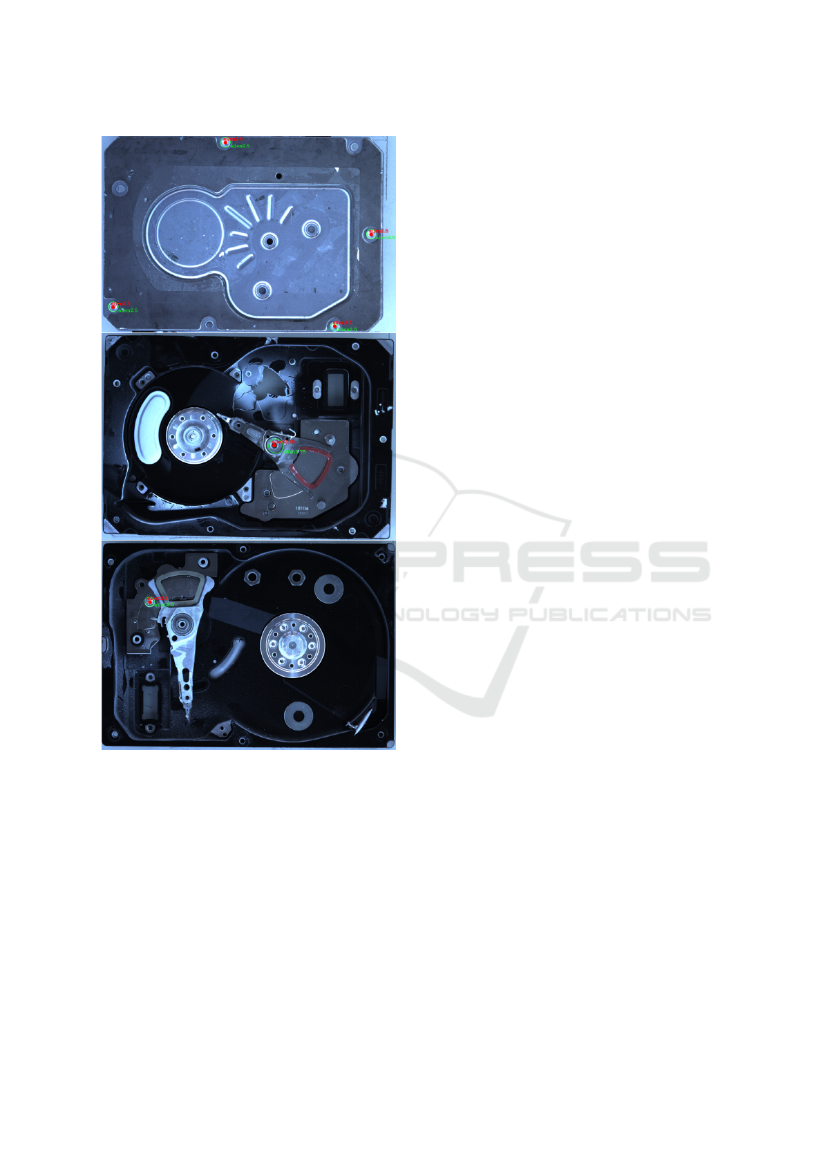
Figure 1: We present a universal, extendable, RGB based

screw head classiﬁer scheme which is engineered for auto-

mated disassembly tasks. Our scheme uses a Hough trans-

form and two state-of-the-art deep convolutional neural net-

works. Green circles represent predicted screw type, red dot

and font represent the ground truth.

In this paper, a visual screw head classiﬁcation

scheme based on a combination of deep learning

methods empowered with classical computer vision

methods is proposed. The proposed scheme can be

seen as an extension of a previous scheme devel-

oped by us (Yildiz and W

org

otter, 2019) to detect

screws. We take the work even further now by mak-

ing it able to classify the screw type and size. We

use the well known Hough transform to ﬁrst gener-

ate screw-candidates (screws and circular artefacts),

which are then ﬁltered out by our previous screw de-

tector model, yielding only screws. Afterward, we

feed the screws into our DCNN powered classiﬁer,

chosen via our experimental evaluation of the top

state-of-the-art models. The scheme can account for

any type of screw size and type as long as the user

collects enough data in the ofﬂine mode for train-

ing. As it was in our previous work, we keep the

feature of data collection. Contrary to state-of-the-

art techniques, which require users to ﬁnd datasets

from search engines for their speciﬁc requirements

(viewpoint, height, etc.), we let users create their own

datasets, given the device and camera. This mitigates

the problem of ﬁnding speciﬁc datasets for screw

types and sizes, and ensures high accuracy for the net-

work.

Therefore, the most signiﬁcant contribution of this

paper is the fusion of features acquired from classical

computer vision methods and the deep learning model

that trains on the data collected by the user in a semi-

automated way. To our knowledge, we are the ﬁrst to

utilise this kind of fusion to classify 12 different screw

head types.

We examine the performance of our proposed

scheme in different situations and the extent of gener-

alization for effective automation and robotics usage

in disassembly. For our experiments, we have col-

lected approximately 35000 training images of differ-

ent screw head types and sizes. Additionally, 50 sam-

ple scenes of various disassembly stages of computer

hard drives were collected to test the pipeline.

2 RELATED WORK

There have been several studies researched under the

topic of automated disassembly (Weigl-Seitz et al.,

2006; Dr

oder et al., 2014; Wegener et al., 2015) which

yielded some schemes (Elsayed et al., 2012; Pomares

et al., 2004; Bdiwi et al., 2016; B

uker et al., 2001)

for automating certain processes. However, these

schemes do not generalize and pose as universal solu-

tions for the problem of classiﬁcation of screw heads.

Basically, the problem of screw head classiﬁcation is

not even addressed yet by the community. There are

some works that involve template matching methods

to ﬁnd the screws on metal ceiling structures for dis-

mantling of certain objects (Ukida, 2007). However,

template matching operates on a ﬁxed template that

looks for a pixel-level match with the target, making

it an extremely undesirable paradigm for cases where

lightening or the object’s color changes. It is there-

fore impossible to account for all screw heads of all

ROBOVIS 2020 - International Conference on Robotics, Computer Vision and Intelligent Systems

colors, sizes, lightening conditions by using template-

matching based methods, making it an impossible

scheme for automated disassembly. An interesting at-

tempt came with the goal of detecting M5 bolts on

battery joints in electric vehicle battery disassembly

routines (Wegener et al., 2015). Using a Haar-type

cascade classiﬁer trained on cropped images of M5

bolts, adding false positives detected from the clas-

siﬁer under negatives, the authors were only able to

achieve 50% detection accuracy for only one type of

bolts. Such low accuracy does not constitute a viable

solution for a disassembly routine, thus making the

method impractical for industrial use.

The last work we would like to mention also fo-

cused on autonomous disassembly of electric vehi-

cle motors (Bdiwi et al., 2016). In this work, screws

found on electric vehicle motors were detected using

an RGB-D sensor (Kinect) (Zhang, 2012). Although

the proposed algorithm is scale, rotation, and transla-

tion invariant, it heavily relies on traditional computer

vision methods such as Harris corner detection and

HSV image analysis. It is a well known fact that these

methods are easily affected by the lighting conditions

and do not generalize. Another shortcoming is the

fact that they require a depth image from the RGB-D

sensor to remove false positives such as holes, which

adds computational load, yet again for merely detect-

ing a screw, not classifying its type and size.

Thus, it seems that there is still a substan-

tial lack in generalizable, device and environment-

independent methods to detect and classify screw

heads, which can be used in automated disassembly

processes.

3 METHOD

In this section we explain each block in our pipeline.

However, before doing that, we would like to inform

the reader about the setup our scheme requires. We

propose a setup in which the camera faces the device’s

surface perpendicularly. The distance between the de-

vice and the camera was 75 cm, however, depending

on the size of the device, this distance may change.

Since we worked with computer hard drive screws,

75 cm was a suitable height.

We keep the pipeline we inherit from our previous

work(Yildiz and W

org

otter, 2019), and add a classiﬁ-

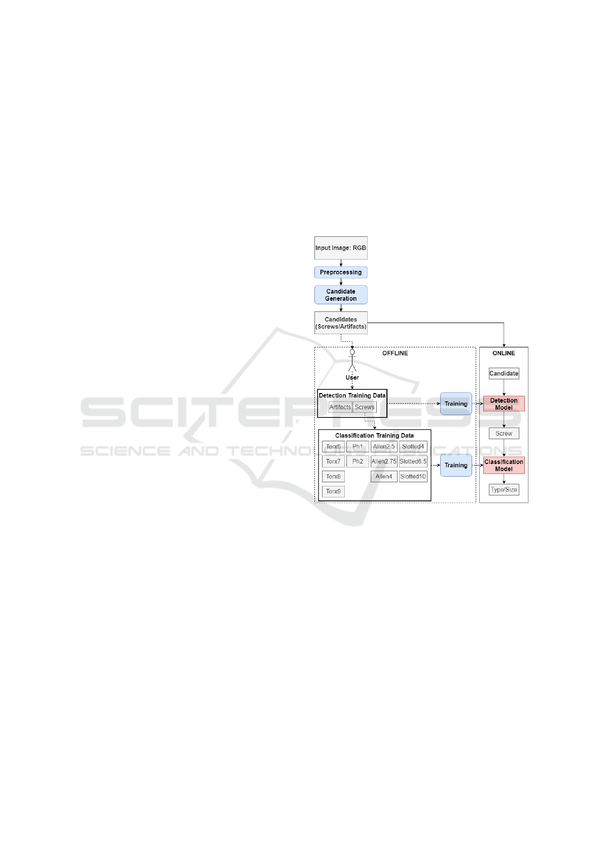
cation block to it, as illustrated in Fig. 2. Our previous

work enables the user to collect training data by crop-

ping circular candidates from the scene. The cropped

circular candidates are then to be divided into their

respective classes (artifact, Torx8, Ph2, Slotted6.5,

Allen2.75, etc.) by a human.

Afterward, ﬁrst the detector model can be trained

to classify screws from artefacts (circular non-screws

structures), as we explained in our previous work

(Yildiz and W

org

otter, 2019). Having deployed a

model that can differentiate screws from artefacts,

now we can train and deploy our new classiﬁer, that

can classify 12 different types of screw heads. Our

scheme then marks and returns the type/size informa-

tion and locations of the screws seen in the image.

3.1 Preprocessing

Figure 2: The pipeline in our scheme is composed of online

and ofﬂine stages. Online stage employs models to differen-

tiate screws from artefacts, as well as to classify the screws.

The preprocessing step is directly taken from our pre-

vious work (Yildiz and W

org

otter, 2019), where clas-

sical computer vision is ﬁrst used to crop the image

to only the region where the device is visible, and

grayscale it.

3.2 Candidate Generation

E-Waste is a vast category of devices with different

structures and materials. A possible screw head clas-

siﬁer should therefore account for all or most of the

screws encountered in the disassembly domain. In

order to come up with a scheme that has reasonable

levels of generalisation ability. We analyzed differ-

ent types of screws found in the domain of E-Waste.

To make sure that our method will cover the most en-

DCNN-based Screw Classiﬁcation in Automated Disassembly Processes

countered and conventionally used screw types found

in this domain, we have consulted experts from the

disassembly plant in cooperation with our university

and agreed on 12 types of screw heads such as dif-

ferent sizes of Torx, Philips, Slotted and Allen heads.

We assessed various electronic devices, which can be

found in huge numbers nowadays in E-Waste, such as

computer hard drives, DVD players, gaming consoles

and many more. As anticipated, we concluded that

almost all screws in this domain are circular, which is

the natural geometry of these objects and represents

the central feature to be utilised to detect a screw ob-

ject. Fig. 3 illustrates samples of screw types/sizes

classiﬁed in our dataset. It must be underlined that

there are also non-circular screws manufactured, how-

ever, those are few and we found no such screws in the

devices of interest in the disassembly plant we coop-

erate with. We therefore based our method on ﬁrst

ﬁnding circular structures in the images. Clearly, not

every circular structure is a screw, for example stick-

ers, holes, transistors, etc. exist, which are also circu-

lar, but not screws. Nevertheless, circular structures

provide us with priors for screws and the ﬁrst step of

our method is to collect those screw-candidates.

Figure 3: Screw types encountered during the disassembly

of various electronic devices found in E-Waste. Last row

depicts artefacts that count as another type in classiﬁcation.

We use the base candidate generator from our pre-

vious work (Yildiz and W

org

otter, 2019), in order

to collect candidates. We run our program in ofﬂine

mode and rely on the Hough Transform for candidate

detection. This is a standard computer vision method

for circle detection (Duda and Hart, 1971) and shall

not be explained here. Differing from the standard

Hough Transform here we use a version, relying on

the so called Hough Gradient (of the OpenCV library

(Bradski and Kaehler, 2008)). This version uses the

gradient information of the edges that form the cir-

cle. We refer the reader to the handbook published

by the creators of the aforementioned library for fur-

ther implementation details on the algorithm of the

Hough Gradient. It should be noted that after col-

lecting our candidates, we then switch back to RGB

from grayscale, since our classiﬁers operate far better

in colored images than in grayscaled ones.

3.3 Training the Classiﬁers

As mentioned before, the user manually separates

screw types and artifacts by which a classiﬁer can be

trained using these positive and negative examples as

training data. In Fig. 3 types of screw heads and ar-

tifacts taken from various devices found in E-Waste

are shown. In general, these screws are found in other

device-classes and, thus, the resulting training set can

be transferred also to other devices. In that case, how-

ever, one has to increase the number of samples to

account for more types of screws.

We have investigated state-of-the-art classiﬁers

found in the literature and we picked the three top-

performing ones for comparison at the end. These

networks, to our experience, were performing toler-

ably good given a not so large dataset for a speciﬁc

device-class (hard drives of any size). Finally, we de-

cided to evaluate EfﬁcientNets (Tan and Le, 2019),

ResNets (He et al., 2016), DenseNets (Huang et al.,

2017), scoring top accuracies on the ImageNet (Deng

et al., 2009). Additionally, EfﬁcientNets have been

used in the latest works (Xie et al., 2019) in pur-

suit of improving ImageNet classiﬁcation, by using a

new self-traning method called Noisy Student Train-

ing. Inspired by this effort, we chose EfﬁcientNetB2.

Our strategy to evaluate the networks is described

as follows. We go by the standard procedure for trans-

fer learning: cutting the pre-trained model on the last

convolutional layer and adding a new sequence of lin-

ear layers called the head. We use this head architec-

ture for all models we explore. In the ﬁrst 10 epochs,

we train only the added ﬁnal layers of the model by

freezing all convolutional layers, not allowing any up-

dates to their weights. Afterward, we unfreeze all lay-

ers and train the entire network. We ﬁnd it useful to

use differential learning rates at this stage. It is not de-

sired to change the early layers of the models as much

as the later ones, therefore lower learning rates are

used in the ﬁrst layers and higher ones in the end. Us-

ing the Adam optimizer (Kingma and Ba, 2014) with

the learning rate of 1 ×10

−5

. Figure 4 illustrates the

model architecture we use. Here, the term ”Block” is

a higher abstraction used for group of layers.

To further reduce overﬁtting and to come up with

a model that can generalize, we applied an additional

data augmentation step. There are several data aug-

mentation operations we applied to introduce more

variety in the data such as rotation, brightness and

contrast.

ROBOVIS 2020 - International Conference on Robotics, Computer Vision and Intelligent Systems

Figure 4: Head architecture of the model.

4 EXPERIMENTAL EVALUATION

We conducted several experiments on the test data we

collected. Out of the top three state-of-the-art classi-

ﬁers, we picked the best performing one, namely Efﬁ-

cientNetB2 -one of the best performing models given

Noisy Student weights- and used it in the pipeline

seen in Fig. 2. Below we also provide details of

the experimental evaluation and present our justiﬁca-

tion for our decision of picking the one we use in our

pipeline.

4.1 Experimental Environment

For the evaluation of the screw classiﬁers, we col-

lected a dataset of over 20000 samples and split it

into training and validation sets with the ratio of 2:1.

We use a computer with Intel Core i7-4770 CPU @

3.40GHz, 16GB of RAM with GeForce GTX Titan X

graphics card to train the classiﬁers. For evaluation of

the performance of our entire pipeline, we collected

approximately 50 hard drive images containing over

500 screw-like elements as the test set the model has

never seen before.

4.2 Experimental Metrics

Our pipeline is composed of two main blocks, namely

the Hough circle detector and our classiﬁer, Efﬁcient-

NetB2. It is required to assess the detection as well

as the classiﬁcation abilities of the entire pipeline.

To this end, we went by the following strategy: We

ﬁrst annotated the test images, each having only one

hard drive with top-down view. These images contain

drives with or without screws, by which the Hough

circle ﬁnder could be assessed. We annotated these

scene images by marking screws with squares, which

would form our ground truth for assessing the Hough

Table 1: Accuracy of the state-of-the-art models with huge

variation of hyperparameters. Highlighted ones are the top

three performing ones.

Model Grayscale Size Loss Acc. Min. Acc. F1 Transfer Learning

EfﬁcientNetB2A No 256 0.1187 0.968 0.79 0.97 Noisy Student

EfﬁcientNetB2A No 64 0.2144 0.936 0.78 0.93 ImageNet

EfﬁcientNetB2A No 128 0.1871 0.951 0.85 0.95 ImageNet

EfﬁcientNetB2A Yes 128 0.2199 0.948 0.67 0.94 ImageNet

EfﬁcientNetB3A Yes 64 0.2072 0.937 0.75 0.93 ImageNet

EfﬁcientNetB3A No 64 0.2051 0.939 0.74 0.94 ImageNet

DenseNet121 No 128 0.1415 0.961 0.81 0.96 ImageNet

DenseNet121 Yes 128 0.1489 0.957 0.74 0.95 ImageNet

DenseNet121 No 64 0.1896 0.937 0.72 0.93 ImageNet

DenseNet121 No 64 0.2306 0.934 0.71 0.93 ImageNet

DenseNet201 No 256 0.1170 0.966 0.79 0.96 ImageNet

ResNet34 No 128 0.1538 0.955 0.80 0.95 ImageNet

ResNet34 Yes 128 0.2026 0.951 0.69 0.95 ImageNet

ResNet50v2 No 256 0.1732 0.942 0.73 0.94 ImageNet

circle ﬁnder’s accuracy. We went by the standard

VOC evaluation (Everingham et al., 2010) and we

found our Hough circle detector to work with 0.783

mean IoU with the optimal parameters found for our

setup. IoU here refers to what amount of screw region

is correctly detected by the Hough circle ﬁnder. If the

detected region for a screw is below 70% it’s bound

to result in bad prediction for both detection and clas-

siﬁcation. It must be also noted that our pipeline is

limited by the accuracy of Hough, since if the circle

ﬁnder cannot catch the circle, then the classiﬁer’s ac-

curacy does not matter at all. The accuracy of Hough

circle detection can vary depending on the parame-

ters of the function such as min/max radius, min/max

threshold. Inevitably, ﬁnal accuracy of our pipeline

can be calculated as follows:

Acc Pipeline = Acc CircleDetector ∗Acc Classi f ier

For the evaluation of the classiﬁer, we consider the

standard metrics of loss, accuracy, min accuracy and

f1 score.

4.3 Experimental Results

We summarize the experimental results with regards

to performance of each classiﬁer against the valida-

tion set in Table 1. Note that we are selecting what

model to use in this part of our experiments. Using

the test dataset would cause overﬁtting of the hyper-

parameters.

From the collected results in Table 1, one can con-

clude the following: All of the investigated models

achieve very high accuracy - over 90% on the test-

ing data, with the model EfﬁcientNetB2 scoring the

highest min. accuracy of 85% among single models.

Additionally, we emphasize that augmentation strat-

egy plays a pivotal role in the classiﬁer accuracy. Es-

pecially for circular objects, rotation guarantees that

the traning data accounts for screws that are rotated

for each angle. Using the Albumentations (Buslaev

et al., 2020) library applied a rotation of 360 degrees,

horizontal and vertical ﬂips, as well as brightness and

contrast changes.

DCNN-based Screw Classiﬁcation in Automated Disassembly Processes

Figure 5: Confusion matrix acquired through our experi-

ments.

We then employ the ﬁnal model in our pipeline

and evaluate it on our test dataset. Fig. 6 shows the

precision-recall curve of our classiﬁer, whereas Fig. 5

illustrates the confusion matrix. Our pipeline achieves

an AP of 0.757. The reason why our classiﬁer accu-

racy is higher than our AP is due to the Hough cir-

cle ﬁnder, which succeeds by approximately 75% of

the time, limiting our pipeline’s overall AP. This can

be mentioned as the only limitation of our pipeline.

Fig. 7 illustrates the detection and classiﬁcation of the

screws found on a Hitachi Deskstar 3.5” hard drive

during the disassembly.

Figure 6: Precision-Recall curve for the ﬁnal model for our

classiﬁer.

5 DISCUSSION AND

CONCLUSIONS

In this study we tackled the fundamental problem

of screw head classiﬁcation in disassembly environ-

ments. The problem itself is a challenging one, since

screw heads have variable sizes, types and not every

electronic device has the same type of screw heads.

We proposed a model, which is based on the Hough

transform and two DCNNs. Our proposal was the ex-

tension of the previous work we published, where the

scheme lets user to collect as much as data he/she

desires from a device. Given that the user creates

the ground truth classiﬁcation (i.e., separates the col-

lected screw data into their respective type and size

categories), our model is able to hit very high F1 score

of 97%, whereas with Hough we found the optimal

parameters to hit 78% IoU for screw regions. The re-

sults had been quantiﬁed with hard drive devices of

different models and sizes, which have different sizes

and types of screws as documented by the experimen-

tal evaluation results of our scheme. Additionally,

we acquired screws from other devices and inserted

them into the scene to test the generalization ability

of the pipeline, achieving promising results as well.

The data set as well as the implementation are to be

published to facilitate further research

As future work, we note that Hough circle ﬁnder

can be employed in a better way. An alternative to

our current strategy with Hough circle ﬁnder would

be shifting of detected circle ROI to conduct dynamic

region correction in order to hit higher IoU. This is

due to the fact that candidates suggested by Hough

may be cut off in a way to mislead the classiﬁer.

Note that all the misclassiﬁcations apart from the

intra-class ones (e.g., Torx6/Torx8) are empirically

found to be a direct result of how Hough cuts re-

gions. In some cases the artefacts are found as

Allen2.75, which, however, is a strongly valid clas-

siﬁcation and detection by the classiﬁers since the

candidate cropped by the Hough circle resembles an

Allen screw, and, thus the classiﬁer claims so. The

suggested approach therefore could provide tangible

results by improving the cropping of candidates, how-

ever, it is a different research topic altogether, and,

mostly lies in the area of algorithm building.

https://drive.google.com/drive/folders/

1VFrF7B1FXPTgJRpu8rcnxJFRRKiT2ljY?usp=sharing

ROBOVIS 2020 - International Conference on Robotics, Computer Vision and Intelligent Systems

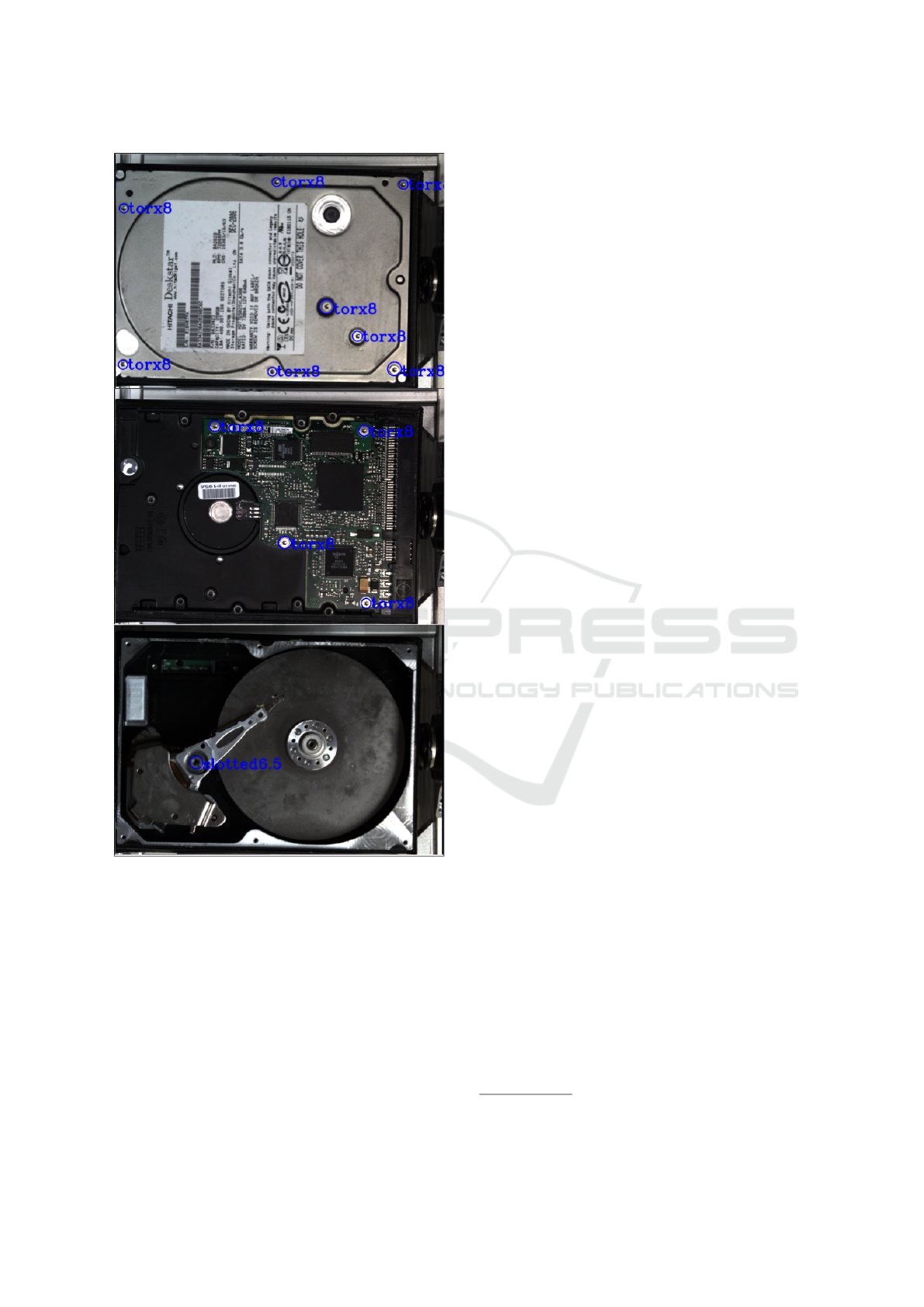
Figure 7: Classiﬁcations of detected screws during the dis-

assembly of a hard drive. All screw types are found cor-

rectly.

ACKNOWLEDGMENTS

The research leading to these results has received

funding from the European Union’s Horizon 2020

Research and Innovation programme (H2020-ICT-

2016-1, grant agreement number 731761, IMAGINE;

https://imagine-h2020.eu/). We would like to also ex-

press our gratitude to the disassembly plant we coop-

erated with, namely Electrocycling GmbH

, for their

continuous support throughout our investigation.

REFERENCES

Bdiwi, M., Rashid, A., and Putz, M. (2016). Au-

tonomous disassembly of electric vehicle motors

based on robot cognition. Proceedings - IEEE In-

ternational Conference on Robotics and Automation,

2016-June(July):2500–2505.

Bradski, G. and Kaehler, A. (2008). Learning OpenCV:

Computer vision with the OpenCV library. ” O’Reilly

Media, Inc.”.

uker, U., Dr

ue, S., G

otze, N., Hartmann, G., Kalkreuter,

B., Stemmer, R., and Trapp, R. (2001). Vision-

based control of an autonomous disassembly station.

Robotics and Autonomous Systems, 35(3-4):179–189.

Buslaev, A., Iglovikov, V. I., Khvedchenya, E., Parinov, A.,

Druzhinin, M., and Kalinin, A. A. (2020). Albumen-

tations: fast and ﬂexible image augmentations. Infor-

mation, 11(2):125.

Deng, J., Dong, W., Socher, R., Li, L.-J., Li, K., and Fei-

Fei, L. (2009). Imagenet: A large-scale hierarchical

image database. In 2009 IEEE conference on com-

puter vision and pattern recognition, pages 248–255.

Ieee.

oder, K., Raatz, A., Herrmann, C., Wegener, K., and An-

drew, S. (2014). Disassembly of Electric Vehicle Bat-

teries Using the Example of the Audi Q5 Hybrid Sys-

tem. Procedia CIRP, 23:155–160.

Duda, R. O. and Hart, P. E. (1971). Use of the hough trans-

formation to detect lines and curves in pictures. Tech-

nical report, SRI INTERNATIONAL MENLO PARK

CA ARTIFICIAL INTELLIGENCE CENTER.

Elsayed, A., Kongar, E., Gupta, S. M., and Sobh, T. (2012).

A robotic-driven disassembly sequence generator for

end-of-life electronic products. Journal of Intelli-

gent and Robotic Systems: Theory and Applications,

68(1):43–52.

Everingham, M., Van Gool, L., Williams, C. K., Winn, J.,

and Zisserman, A. (2010). The pascal visual object

classes (voc) challenge. International journal of com-

puter vision, 88(2):303–338.

He, K., Zhang, X., Ren, S., and Sun, J. (2016). Deep resid-

ual learning for image recognition. In Proceedings of

the IEEE conference on computer vision and pattern

recognition, pages 770–778.

Huang, G., Liu, Z., Van Der Maaten, L., and Weinberger,

K. Q. (2017). Densely connected convolutional net-

works. In Proceedings of the IEEE conference on

computer vision and pattern recognition, pages 4700–

4708.

Jahanian, A., Le, Q. H., Youcef-Toumi, K., and Tset-

serukou, D. (2019). See the e-waste! training visual

intelligence to see dense circuit boards for recycling.

In Proceedings of the IEEE Conference on Computer

www.electrocycling.de

DCNN-based Screw Classiﬁcation in Automated Disassembly Processes

Vision and Pattern Recognition Workshops, pages 0–

Kahhat, R., Kim, J., Xu, M., Allenby, B., Williams, E., and

Zhang, P. (2008). Exploring e-waste management sys-

tems in the united states. Resources, conservation and

recycling, 52(7):955–964.

Kingma, D. and Ba, J. (2014). Adam: A method for

stochastic optimization. International Conference on

Learning Representations.

Pomares, J., Puente, S. T., Torres, F., Candelas, F. A.,

and Gil, P. (2004). Virtual disassembly of products

based on geometric models. Computers in Industry,

55(1):1–14.

Solomon, R., Sandborn, P. A., and Pecht, M. G. (2000).

Electronic part life cycle concepts and obsolescence

forecasting. IEEE Transactions on Components and

Packaging Technologies, 23(4):707–717.

Tan, M. and Le, Q. V. (2019). Efﬁcientnet: Rethinking

model scaling for convolutional neural networks.

Ukida, H. (2007). Visual defect inspection of rotating screw

heads. In SICE Annual Conference 2007, pages 1478–

1483. IEEE.

Wegener, K., Chen, W. H., Dietrich, F., Dr

oder, K., and

Kara, S. (2015). Robot assisted disassembly for the

recycling of electric vehicle batteries. Procedia CIRP,

29:716–721.

Weigl-Seitz, A., Hohm, K., Seitz, M., and Tolle, H. (2006).

On strategies and solutions for automated disassem-

bly of electronic devices. International Journal of Ad-

vanced Manufacturing Technology, 30(5-6):561–573.

Xie, Q., Luong, M.-T., Hovy, E., and Le, Q. V. (2019). Self-

training with noisy student improves imagenet classi-

ﬁcation.

Yildiz, E. and W

org

otter, F. (2019). Dcnn-based screw de-

tection for automated disassembly processes. In 2019

15th International Conference on Signal-Image Tech-

nology & Internet-Based Systems (SITIS), pages 187–

192. IEEE.

Zhang, Z. (2012). Microsoft kinect sensor and its effect.

IEEE multimedia, 19(2):4–10.

ROBOVIS 2020 - International Conference on Robotics, Computer Vision and Intelligent Systems