Computer Modeling of the Dynamics of Interregional Freight

Transport Depending on Macroeconomic Indicators

Maksim Tatarintsev

, Petr Nikitin

and Sergey Korchagin

Department of Data Analysis and Machine Learning, Financial University under the Government of

the Russian Federation, Shcherbakovskaya, 38, Moscow, Russian Federation

Keywords: Analysis of Macroeconomic Indicators, Dynamics of Freight Traffic, Freight Turnover Assessment,

Forecasting, Import, Export, GDP, GNI, Graph, Correlation Matrix, Correlation-regression Analysis.

Abstract: The purpose of this research is to consider various macroeconomic indicators of world regions(North America,

South America, Europe, Mediterranean, Persian Gulf, CIS, South Africa, Central America, West Africa, East

Africa, East Asia, South Asia, Southeast Asia, Oceania, Australia) and federal districts in the Russian

Federation (Central, North-western, Southern, North Caucasian, Volga, Ural, Siberian, Far Eastern), visualize

the received data, determine their impact on the volume of freight traffic between the designated zones,

identify patterns with the help of which we could carry out various kinds of forecasting. Further, it is necessary

to carry out direct forecasting for several products of the selected industry, applying the necessary math model.

1 INTRODUCTION

It's no secret that interregional trade is important in

the global economy. Even though each state is unique,

the countries within certain zones have somewhat

similar socio-economic and physical-geographical

characteristics. Based on this kind of "kinship", 15

regions of the world can be conditionally defined:

East Africa, West Africa, Central America, South

Africa, Oceania, Mediterranean, CIS, Persian Gulf,

South America, Southeast Asia, South Asia, Europe,

Australia, East Asia, North America.

Each of these zones has completely different

infrastructure, and, speaking directly about our topic,

macroeconomic indicators that are very different

from each other, which stimulate the active

development of interregional trade.

In addition to the global dynamics in the field of

freight traffic and their impact on the economic

indicators of the regions, it is necessary to highlight

trends and relationships in a country. The Russian

Federation was chosen for the research as one of the

most geographically vast and economically

interesting countries in the world.

https://orcid.org/0000-0003-1783-9411

https://orcid.org/0000-0001-8866-5610

https://orcid.org/0000-0001-8042-4089

In a country of 8 major districts: Central Federal

district, North-western Federal district, Southern

Federal district, North Caucasian Federal district,

Volga Federal district, Ural Federal district, Siberian

Federal district and Far Eastern Federal district. For

each of these regions, we selected key economic

indicators for a detailed analysis and identification of

various interesting patterns that allow us to draw

concrete conclusions about the direct impact of

macroeconomic indicators on the volume of cargo

flows both in these zones and in the whole country

Thus, the article will consider: the dynamics of

cargo flows between the selected regions,

macroeconomic indicators of the regions, as well as

their direct influence on each other; the relationship

between freight turnover within the districts of the

Russian Federation and their socio-economic

characteristics. Another important task is to be able to

predict in the short term how the volume of selected

cargo will change in 2020. For this, a special

mathematical algorithm will be used.

Tatarintsev, M., Nikitin, P. and Korchagin, S.

Computer Modeling of the Dynamics of Interregional Freight Transport Depending on Macroeconomic Indicators.

DOI: 10.5220/0010390912491257

In Proceedings of the 13th International Conference on Agents and Artiﬁcial Intelligence (ICAART 2021) - Volume 2, pages 1249-1257

ISBN: 978-989-758-484-8

 2021 by SCITEPRESS – Science and Technology Publications, Lda. All r ights reserved

1249

2 IMPACT OF CARGO FLOWS

ON THE MACROECONOMIC

INDICATORS OF THE WORLD

REGIONS

2.1 Analysis of the Mean Nominal GDP

of the World Regions

Gross domestic product (GDP) is the most important

macroeconomic indicator, which can be understood

as the value of all goods and services produced on the

territory of the country. There is another important

characteristic that, along with GDP, reflects the

degree of development of a country. Gross national

income (GNI) is defined as the sum of GDP and the

balance of primary income (summing up the income

of citizens received from abroad, subtracting funds

taken out of the country by foreigners). To analyse

entire macro-regions, it is necessary to determine the

characteristics by which these districts will be further

investigated. So, the mean nominal gross domestic

product and gross national income were selected.

They were calculated as the arithmetic mean of the

corresponding indicators of all countries located in

this zone.

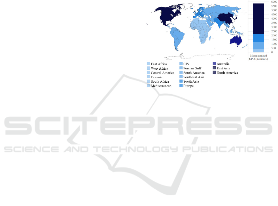
So, in Fig.1 shows a heat map of the world, where

each of the 15 regions is highlighted in colour,

reflecting the value of the average nominal GDP in

this zone in comparison with others. Data for

modelling was taken from. The most economically

developed macro-regions are North America and East

Asia with an average GDP of 5896 billion USDs and

2766 billion USD, respectively. Australia also ranks

high with a GDP of 1376 billion $. Of course, you

need to understand that there are countries that have

a very developed economy, but due to the fact that the

region is dominated by countries that have a low

GDP, the average indicator is decreasing. For

example, the United Kingdom, France and Germany

have a GDP in 2019 more than 2,500 billion USD. but

taking into account some other countries that have

this indicator more than five times less, it turns out

that Europe, as one of the most comprehensively

developed parts of the world, in comparison with the

leading macro-regions in this characteristic, has a

nominal gross domestic product equal to $ 659

billion. But if we consider some other countries that

have this indicator more than five times less, it turns

out that Europe, as one of the most comprehensively

developed parts of the world, in comparison with the

leading macro-regions in this characteristic, has a

nominal gross domestic product equal to 659 billion

USD.

The situation of Africa is not surprising.

Unfortunately, most of the countries of this continent

have a very underdeveloped economy, which is

proved by extremely low average GDP figures: South

Africa - $ 82.5 billion, East - $ 26 billion, West - 34.5

billion $.Many CIS countries are economically

developed at the same level. But the Russian

Federation stands out a lot: its GDP is 1,638 billion $

in 2019.

Figure 1: Mean nominal GPD of world regions (million $).

Python heat map implementation for East Africa:

pip install pygal

import pygal

import numpy

from pygal.style import Style

custom_style = Style( colors =

('#96c5f1'))

worldmap = pygal.maps.world.World(style

= custom_style)

worldmap.title = ' Mean nominal GPD of

world regions (million $).'

worldmap.add('East Africa',

['bi','dj','zm','zw','ke','mu','mg','mw

','mz','rw','sc','so','sd','tz','ug','e

r','et'])

2.2 Analysis of the Mean GNI of the

World Regions

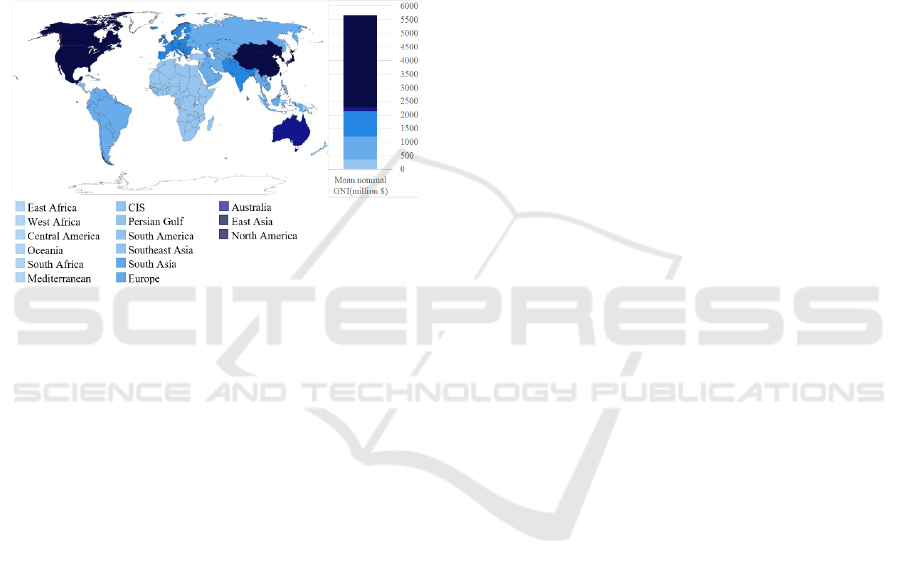
It is advisable to further consider the average GNI in

different regions of the world (fig. 2) and understand

how this characteristic differs from the previously

considered indicator. The overall situation has not

changed much: in the top three developed economic

regions are still North America with an mean GNI of

5729 billion $, East Asia - 2764 billion $, and

Australia - 1346 billion $.

Countries of Africa and Oceania have the worst

indicators-less than 70 billion $. The initial

conclusions before the analysis were as follows: in

ICAART 2021 - 13th International Conference on Agents and Artiﬁcial Intelligence

1250

countries where most of the income is exported

abroad, GNI is less than GDP. On the contrary, if

citizens of a country have high incomes in companies

in other countries, then GNI will exceed GDP.

In practice, the previously made conclusions were

confirmed. A while the difference between gross

domestic product and gross national income may be

significant in theory, in practice it turned out to be

insignificant. For example, if the mean GDP in

Europe is 659 billion USD, the mean GNI is 682.8

billion USD. Relative to these amounts, the difference

is small, but noticeable and is the highest among all

the districts considered.

Figure 2: Mean GNI of world regions (million $).

2.3 Analysis of Cargo Flows between

World Regions

In order not to be unfounded, let's move on to the

analysis of freight traffic between the world macro-

regions. Fig. 3 and Fig. 4 show graphs reflecting the

import and export of all goods between the regions in

monetary terms. The 15 regions into which we united

all states earlier are now presented in the form of 5

larger zones.

The most promising is cooperation between

America and Asia, which can be explained by their

developed economic and trading system. Indeed,

paying attention to the mean nominal GDP and mean

GNI that we examined earlier, it becomes clear that

they are indicators for high trade between these

macro-regions. It should be noted that the import of

products from Asia to America (1611million USD) is

almost 2 times more than in the opposite direction

(980 million USD). Why is this happening?

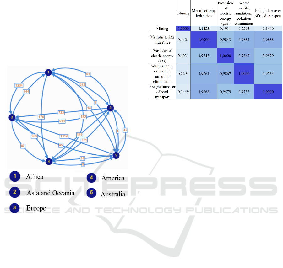
I propose to carefully consider Fig. 5. The total

tonnage of freight turnover between Asian countries

and the rest of the world tells us that China, Japan,

India, Korea and other large manufacturing countries

in Asia have a powerful resource base - no other

macro-region has such a volume of goods supplied to

other zones: In 2019, more than 350 million tons of

agricultural products alone were supplied, fuel - more

than 1.24 billion tons, metals and minerals - more

than 700 million tons. And this is not all the products

exported by Asia.

The trade partnership between the countries of

Europe and America is no less interesting: fertilizers,

metals and minerals, gas, oil are also in great demand

here. The supply of various goods from Europe to

Australia, as two economically developed regions of

the world, is surprising: the weight of the transported

goods in 2019 (Fig. 5) and its monetary equivalent

(Fig. 3 and Fig. 4) is not large.

How can such a commodity exchange

phenomenon be explained? Previously, the analysis

could only be based on economic indicators, but now

it is necessary to consider the geographical location

of the regions: Europe and Australia are among the

most distant trading partners. Therefore, it is much

more profitable for them to look for suppliers in

countries that are closer. This is what happens –

Australia prefers to import goods mainly from Asia

and Oceania. However, why are there deliveries from

Australia to Europe and back at all? This question can

be answered if you pay attention to the types of

products delivered. The basis of trade is coal, which

is not surprising: Australia is a major exporter of this

type of raw material in the world.

It is interesting that African countries with low

macroeconomic indicators supply a lot of goods, for

example, to America (more than a billion tons in

2019). The most exported precious metals, ores and

phosphorites. At the same time, African countries buy

little cargo from other macro-regions. How can this

be explained? The federal budget plays an important

role here. Mauritania, Togo, Eritrea, Burundi,

Lesotho, Swaziland, Liberia and other countries are

among the poorest in the world (GDP less than US $

10 billion). That’s why many states do not have the

ability to purchase goods from abroad.

Trade cooperation between Europe and Asia is no

less important than the rest. Perhaps the most

prominent is the cargo turnover between these macro-

regions. The difference in the quantity of products

delivered between these zones is very noticeable: 213

million tons from Asia to Europe, 721 million tons in

the opposite direction. It is very important to

understand why there are such strong differences in

the volume of deliveries.

To do this, you need to consider the types of

products. The most priority cargoes from Europe to

Asia are forestry products, fossil fuels, agricultural

products, gold, silver and other precious metals,

palladium, platinum.

Computer Modeling of the Dynamics of Interregional Freight Transport Depending on Macroeconomic Indicators

1251

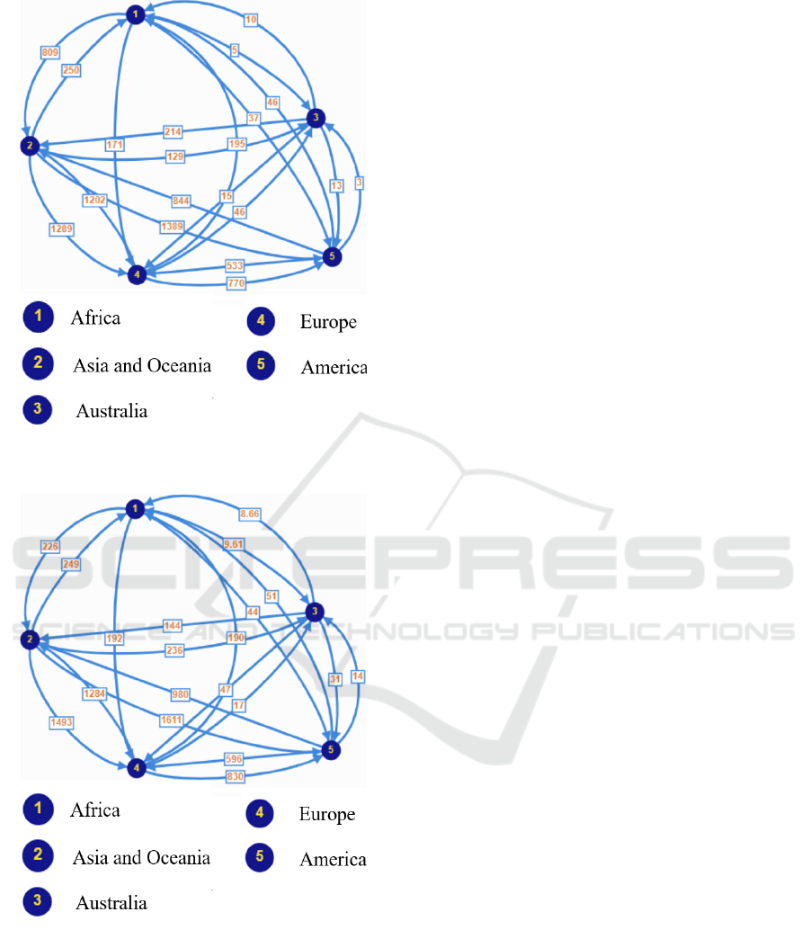
Figure 3: Import of all goods between world regions

(million $).

Figure 4: Export of all goods between world regions

(million $).

If we talk about the opposite direction, the most

common products here are fossil fuels and minerals,

precious metals. Assuming that China is one of the

world's largest gold, silver and other precious metals

mining centers, it was assumed that this type of goods

would occupy an impressive part of the total supply.

In reality it turned out that precious metals are a small

part of the total cargo turnover between the regions,

but Asia places a great emphasis on the supply of this

expensive resource. So, if we consider the monetary

equivalent of exported goods, this indicator is

comparable between both zones (from Asia to

Europe, $ 1,288 million, in the opposite direction, $

1,202 million).

After analyzing the obtained indicators, we can

make a reasonable conclusion that cargo tonnage is

not the only factor that should be considered when

analyzing cargo flows. It is very important to consider

what specific resource is being delivered, because

each product has a different market value. For

example, in our case, the supply of gold and other

precious metals from Asia to Europe is not

comparable in price with forestry products, which

take up most of the supply in the opposite direction.

Thus, cargo turnover directly depends on the

economic development of the cooperating regions,

and the partner States in particular. However, it is

necessary to take into account the geographical

factor: trade relations between Europe and Australia

show us that remote macro-regions can also cooperate

with each other, but due to the strong remoteness of

the zones, we cannot count on a high exchange of

goods. When analyzing cargo transportation between

regions, you need to consider the type of products

delivered: regions that specialize in the production

and processing of any product will always offer their

range to those who need it. In international practice,

this is confirmed by Asian countries, whose products

are in demand on the world market.

3 MUTIAL IMPACT OF CARGO

FLOWS ON

MACROECONOMIC

INDICATORS OF THE

RUSSIAN DISTRICTS

The Russian Federation is a vast country with the big

national resources which has a great economic

potential. Key feature of the country - very convenient

location for trade relations. The country consists of 8

districts: Central Federal district, North- western

Federal district, Southern Federal district, North

Caucasian Federal district, Volga Federal district, Ural

Federal district, Siberian Federal district and Far

Eastern Federal district. Every region has its own

macroeconomic indicators. For the analysis of cargo

flows between districts, the following characteristics

were selected: mining (million rubles), manufacturing

ICAART 2021 - 13th International Conference on Agents and Artiﬁcial Intelligence

1252

industries(million rubles), provision of electric

energy(gas) (million rubles), water supply, sanitation,

pollution elimination (million rubles), the carriage of

goods by road transport organizations of all activities

(million tons), freight turnover of road transport

organizations of all activities (million ton - km), the

turnover of wholesale (retail) trade organizations of

wholesale (retail) trade (million tons),retail trade

turnover (million tons), export and import (million

USD), foreign trade turnover (million USD).

Figure 5: Freight traffic between world regions (million

tons).

In order to determine which of these economic

indicators have the greatest impact on cargo flows

between districts, we construct symmetric correlation

matrix (Table 1). As you know, correlation is

equivalent to an approximate relationship between

any values. The linear coefficient of pair correlation

between characteristics is calculated using the

“CORREL” function program in Microsoft Excel.

All elements of the main diagonal are equal to one

– the correlation of each macroeconomic indicator

with itself. The rest of the cells are filled with

numbers from the limit [-1; 1], which make it possible

to assess the strength of the relationship between

quantities. Based on the scale of the statistician

Chaddock, it can be argued that values close to -1

reflect a strong negative relationship (strong

feedback), to 1 - a strong positive relationship (direct

relationship), close to 0 - no relationship. If the

correlation coefficient is close to 0.5 or -0.5, then the

selected indicators are in moderate dependence.

Table 1: Correlation square matrix.

Therefore, it is necessary: to find such indicators

that are most dependent on the characteristics

associated with cargo transportation (the correlation

coefficient in modulus is close to 1) and to justify the

identified dependencies.

Freight turnover of road transport is highly

correlated with manufacturing industries. Since the

corresponding coefficient is close to 1, then for this

pair of macroeconomic indicators, a direct

relationship can be identified and explained.

Cargo transportation depends on the volume of

output of the chemical, timber, light, food and other

industries, which are key in the manufacturing

industry of the country. Indeed, when the demand for

goods decreases, the number of products produced is

also adjusted. As a result, the volume of cargo

transportation also decreases. On the contrary, with

an increase in the number of products created, it is

necessary to deliver proportionally more goods,

which entails an increase in the volume of cargo

transportation.

The correlation coefficient between freight

turnover of road transport and the provision of

electric energy is also very close to 1. Therefore, a

directly proportional relationship is also noticeable

between these indicators: with increased demand for

electricity, steam or gas, the need for cargo

transportation will also increase. Since provision

refers not only to direct transmission, but also to the

installation and maintenance of devices, the last two

services account for the greatest load associated with

cargo flows. You can show the relationship as

follows: if you need electricity, you need to bring and

install a system of lines, meters, and poles that

transmits energy from point A to point B. In case of

breakdowns or when the warranty period expires, it is

necessary to replace the equipment, that is, to deliver

new equipment. However, if the demand for

Computer Modeling of the Dynamics of Interregional Freight Transport Depending on Macroeconomic Indicators

1253

electricity increases, the volume of cargo flows will

increase, which will be proof of a direct proportional

relationship.

Water supply, sanitation, and pollution

elimination are strongly correlated with road

transport freight turnover, which highlights the

relationship between them. It is obvious that water

distribution for drinking, industrial and other needs is

carried out mainly by road. Road transport also

provides services for the restoration of various areas

that have been affected by pollution. The relationship

is obvious here.

Thus, we were able to find three macroeconomic

indicators that have the greatest impact on cargo

turnover and cargo flows between districts in the

Russian Federation. Based on the stable relationship

between these characteristics, you can make forecasts

that will reflect changes in the volume of cargo flows

when one of the three indicators decrease or increase.

For example, if there is a reduced demand for water

supply due to the rise in the price of provider services,

the volume of cargo flows will significantly decrease

in this area. However, it is not necessary that a similar

situation will occur in the entire district – the lack of

demand for these services is compensated by

increased demand for others.

5 FORECASTING THE EXPORT

VOLUME OF COAL AND

PETROLEUM PRODUCTS

FROM RUSSIAN FEDERATION

We have found that manufacturing industries strongly

affects the volume of cargo flows in the Russian

Federation. Based on this material, we will make a

forecast for the volume of exports of petroleum

products and coal from the country in 2020. There are

many different methods used to predict the volume of

cargo flows. Here are some of them: a method based

on calculating the coefficient of transportability of a

certain group of cargo, a method for predicting cargo

transportation based on specific standards, methods

for predicting the average distance of transportation,

and forecasting the transport and economic balance

We chose correlation-regression analysis. It uses very

clear mathematical tools and a clear algorithm that

works perfectly when predicting characteristics that

primarily have quantitative indicators, considering

the dependence of the effective value on many

factors. Moreover, the method is suitable for working

with time series, which will be discussed later. It is

obvious that the method includes a correlation that

has already been used to establish patterns between

the volume of automobile cargo flows and three types

of macroeconomic indicators, and a regression that

allows reflecting the dependence of the effective

indicator on the factor indicator. The purpose of this

study is to apply the method of correlation- regression

analysis in predicting the volume of cargo flows of

coal and petroleum in the short term (for 2020 year).

I would like to note that a relatively small-time

interval is taken, because this will increase the

accuracy of the forecast made.

So, as a productive factor, we will choose the

volume of petroleum products exported from Russia.

To conduct an analysis for this group, we must

provide data for the retrospective period for the

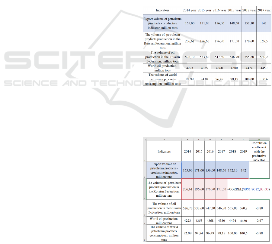
considered influencing factors (Table 2).

Table 2: Indicators required for correlation-regression

analysis by the export volume of petroleum products.

After selecting the necessary statistical data, we

will start calculating linear pair correlation

coefficients using the "CORREL" function in

Microsoft Excel (Table 3).

Table 3: Calculating Pairwise Correlation Coefficient.

ICAART 2021 - 13th International Conference on Agents and Artiﬁcial Intelligence

1254

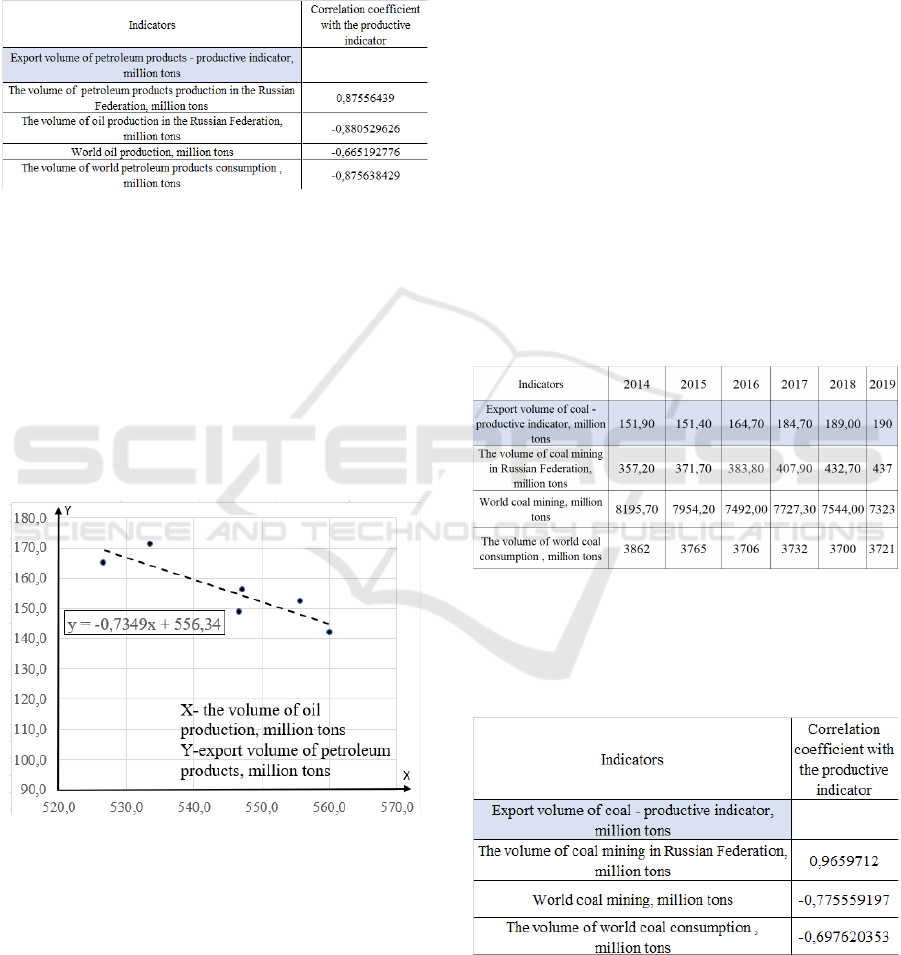
The table 4 shows data on the calculated

correlation coefficients of the expert identified

influencing factors with the indicator volume of

petroleum products exports from the Russian

Federation (million tons).

Table 4: Correlation coefficients of influencing factors.

It’s clear that the most closely related factor to the

performance indicator is the volume of oil production

is the volume of oil mining in the Russian Federation

(modulus of the correlation coefficient 0.88 – on the

Cheddock scale, the degree of correlation is defined

as high, while the relationship is negative). At this

stage, the correlation component is over.

Let's move on to finding the regression equation

that will help you find the predicted value of the

effective factor .To do this, we will plot the

correlation between export volume of petrol products

and the volume of oil mining (Fig. 6).

Figure 6: The field of the correlation dependence.

After plotting the correlation dependence, the

program outputs the regression equation. At the same

time, the coefficient at X (-0.7349) shows the degree

of influence of export volume of petroleum products

on the volume of oil mining, and the free term 556.34

shows what value the resulting value will take if the

factor indicator is not taken into account in the

regression equation (meaning the dependence of

traffic volume on other factors not described in the

model). And the free term 556.34 shows what

quantity the effective value will take if the factor

indicator is not taken into account in the regression

equation (meaning the dependence of the volume of

traffic on other factors not described in the model).

Next, to calculate the forecast traffic volume, we

substitute the prospective value of the influencing

factor (the volume of oil mining) for 2020 into the

resulting regression equation. In the energy strategy

of Russia until 2035 года, compiled by the former

Minister of energy of the Russian Federation A.V.

Novak, the desired value is 525 million tons.

Substituting this value instead of the variable x, we

get 170.5 million tons-the forecast export volume of

petroleum products from the Russian Federation in

2020.

As the next productive indicator, let's take the

Export volume of coal from the Russian Federation

and make a table with data for the period 2014-2019

(Table 5).

Table 5: Indicators required for correlation-regression

analysis by the export volume of coal for 2014-2019 years.

The next step is to calculate the corresponding

correlation coefficients using the program Microsoft

Excel (Table 6).

Table 6: Correlation coefficients of influencing factors.

The table shows that the most dependent factor

with the effective indicator is the volume of coal

mining in the Russian Federation (the value of the

correlation coefficient is 0.97-on the Cheddock scale,

Computer Modeling of the Dynamics of Interregional Freight Transport Depending on Macroeconomic Indicators

1255

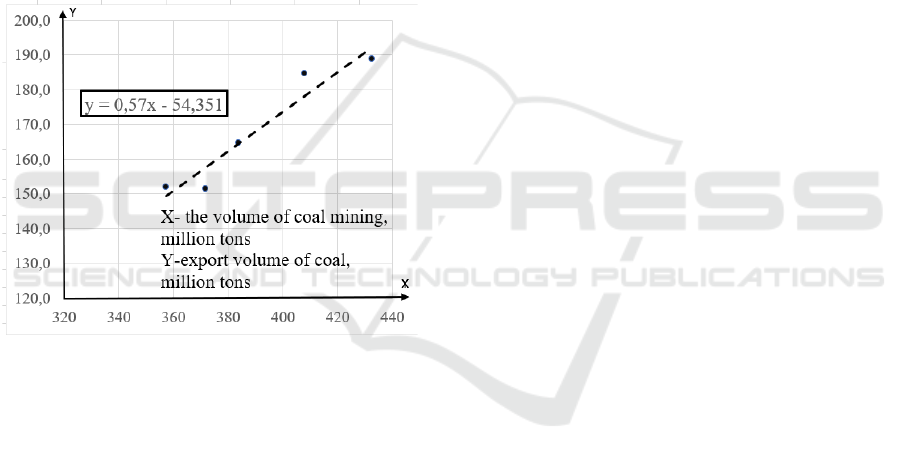
the degree of correlation is defined as a strong

positive.

Тow let's plot the correlation dependence of 1 and

3 indicators (Fig. 7).

We got the regression equation y = 0,57*x-

54,351. To calculate the forecast volume of coal

exported from Russia, substitute the prospective

value of the volume of coal mining for 2020 instead

of the variable x. In the forecast of socio-economic

development of the Russian Federation for the period

up to 2036, compiled by the Ministry of Economic

development of the Russian Federation, the required

value is 420 million tons. Then the Export volume of

coal from the Russian Federation in 2020 will be 185

million tons.

So, formalized methods of predictive

extrapolation are used when predicting certain

processes that can be characterized quantitatively.

Figure 7: The field of the correlation dependence.

When considering the retrospective period, the

trends of the past are considered, analyzed, and the

necessary mathematical methods are applied. This

results in accurate forecast data for a specific

phenomenon. In our research, we used a correlation-

regression algorithm that made it possible to make a

forecast for the selected indicators in the previously

analyzed area. The obtained values - the volume of coal

exports from the Russian Federation in 2020 will be

185 million tons, exports of petroleum products from

the Russian Federation in 2020-170.5 million tons.

6 CONCLUSIONS

So, the article considered various aspects of the

impact of macroeconomic indicators on the volume

of cargo flows.

Firstly, such macroeconomic indicators as the

average nominal gross domestic product (GDP) and

average gross national income (GNI) in each of the

15 selected regions of the world were considered and

analyzed. Next, we examined the volume of cargo

transportation between these zones, correlated it with

the import and export of goods of all types in

monetary terms. As a result, it was concluded that

cargo turnover between regions of the world depends

on many factors. These include the level of economic

development of States, the Federal budget of the

buyer country, the geographical distance of partners,

the type of cargo and its market value.

Secondly, in the Russian Federation, we also

analyzed macroeconomic indicators that could

theoretically be related to the volume of cargo

transportation between districts. In order to identify

dependencies, we have compiled a square correlation

matrix, which was used to identify indicators that

affect the turnover of road transport: output of

products by processing industries, provision of

electric energy, water supply(sanitation) and

elimination of pollution.

Thus, based on these economic characteristics, we

considered situations in which the volume of cargo

turnover between regions of the country may increase

or fall, which marks a success in the field of

interregional forecasting.

Thirdly, we applied the correlation-regression

model and predicted the volume of exports of

petroleum products and coal from the Russian

Federation in 2020. We have deliberately made a

short-term forecast, as this will increase the accuracy

of the forecast. Of course, we must not forget about

the availability of other methods that are actively used

in forecasting. However, our method is particularly

valuable – it allows you to predict the required value

based on quantitative characteristics. The algorithm

also provides the ability to reflect the relationship

between the effective value and influencing factors.

In total, forecasting traffic flows is a very

significant element of the economy. A well-

functioning freight transport system is one of the most

important elements of any successful economy. This

process allows you to: predict the prospects for the

development of the entire system as a whole when

distributing goods in the future; rationally use and

distribute available resources; improve the quality of

transport services, increasing the competitiveness of

the organization; minimize the risk of bankruptcy;

make innovations in the enterprise; improve control

over the processes of transporting goods.

ICAART 2021 - 13th International Conference on Agents and Artiﬁcial Intelligence

1256

REFERENCES

Yang X. et al. Environmental efficiency and equality

embodied in China's inter-regional trade //Science of

The Total Environment. – 2019. – Т. 672. – P. 150-161.

Wu X. F., Chen G. Q. Global overview of crude oil use:

From source to sink through inter-regional trade

//Energy Policy. – 2019. – Т. 128. – P. 476-486.

Lecca P. et al. Upward pressure on wages and the

interregional trade spillover effects under demand‐

side shocks //Papers in Regional Science. – 2020. – T.

99. – № 1. – P. 165-182.

Rajesh P., Karthikeyan M. Data Assimilation of Gross

Domestic Product (GDP) in India Using Stochastic

Data Mining Approach //Journal of Computational and

Theoretical Nanoscience. – 2019. – Т. 16. – №. 4. – P.

1478-1484.

Rana R. H., Alam K., Gow J. Health expenditure and gross

domestic product: causality analysis by income level

//International Journal of Health Economics and

Management. – 2020. – Т. 20. – №. 1. – P. 55-77.

Savoldi A. et al. Gross national income and antibiotic

resistance in invasive isolates: analysis of the top-

ranked antibiotic-resistant bacteria on the 2017 WHO

priority list //Journal of Antimicrobial Chemotherapy.

– 2019. – Т. 74. – №. 12. – P. 3619-3625.

Honig D. Information, power, and location: World Bank

staff decentralization and aid project success

//Governance. – 2020. – Т. 33. – №. 4. – С. 749-769.

Computer Modeling of the Dynamics of Interregional Freight Transport Depending on Macroeconomic Indicators

1257