Filtered Weighted Correction Training Method for Data with Noise

Label

Yulong Wang

1,2,3

, Xiaohui Hu

1,3

and Zhe Jia

School of Computer Science (National Pilot Software Engineering School), Beijing University of Post and

Telecommunications, Beijing, China

Science and Technology on Communication Networks Laboratory, Shijiazhuang, China

State Key Laboratory of Networking and Switching Technology, Beijing, China

Keywords: Noise Label, Noise Filtering, Weighted Correction, Deep Neural Network.

Abstract: To solve the problem of low model accuracy under noisy data sets, a filtered weighted correction training

method is proposed. This method uses the idea of model fine-tuning to adjust and correct the trained deep

neural network model using filtered data, which has high portability. In the data filtering process, the noise

label filtering algorithm, which is based on the random threshold in the double interval, reduces the

dependence on artificially set parameters, increases the reliability of the random threshold, and improves the

filtering accuracy and the recall rate of clean samples. In the calibration process, to deal with sample

imbalance, different types of samples are weighted to improve the effectiveness of the model. Experimental

results show that the propose method can improve the F1 value of deep neural network model.

1 INTRODUCTION

In recent years, machine learning has played an

important role in computer vision, information

retrieval, speech processing, and other scenarios. In

the field of machine learning, a common type of

scenario is to use labeled data to train neural networks

for classification, regression, or other purposes. This

method of learning potential laws through training

models is called supervised learning. In supervised

learning, the learning effect of the model is closely

related to the quality of data labels. Due to the

structural characteristics of the neural network, to

obtain a better learning effect, the amount of training

data needs to reach a certain scale, that is, a large

amount of data, to avoid over-fitting for a small

number of training samples, which leads to the lack

of generalization of the model.

When collecting data, considering the cost factor,

researchers often use methods such as crowdsourcing

tagging, crawling, and external information analysis.

However, the different job occupations and technical

knowledge levels of the marking personnel have led

to uneven marking quality. In addition, external

information analysis methods such as analyzing CDR

information, because the information is easily

tampered with, the reliability cannot be guaranteed,

and the label quality cannot be guaranteed, resulting

in label noise in the data set. These data sets that

cannot guarantee quality and contain label noise are

called noisy data sets.

To sum up, due to the contradiction between the

demand for the amount of data by the neural network

and the cost of manual labeling, the generation of

noisy data sets is an inevitable result of the massive

data collection process (Algan G & Ulusoy I. 2019).

The research on training a more accurate deep neural

network model under the labeled noise data set has

great practical value.

In the past five years, the main research papers on

label noise have increased by multiples (Song H et al.

2020), and the content of these papers covers

theoretical and application research, which reflects

the theoretical research value and practical

application value of label noise learning.

According to the research object, the existing

research can be divided into the following three types.

The first is optimization processing based on training

data, which filters or relabels suspected wrong labels

through clustering, multi-classifier voting, etc., and

uses the cleaned data to train the model to improve

model accuracy (Nicholson B, Sheng SV, Zhang J,

2015); In optimize the processing based on the

Wang, Y., Hu, X. and Jia, Z.

Filtered Weighted Correction Training Method for Data with Noise Label.

DOI: 10.5220/0010577901770184

In Proceedings of the 2nd International Conference on Deep Learning Theory and Applications (DeLTA 2021), pages 177-184

ISBN: 978-989-758-526-5

177

network structure, the model is robust to noise by

optimizing the network structure, such as setting two

identical neural networks to guide each other,

learning the loss value of each other to avoid falling

into overfitting and increasing robustness (Han B,

Yao Q, Yu X. 2018); The third is the optimization

processing based on the loss function, which

constructs a loss function that is robust to label noise,

and reduces the influence of label noise through the

robustness of the loss function itself (Zhang Z,

Sabunc M. 2018; Wang Y, Ma X, Chen Z, et al.

2019). Among them, the optimization of network

structure and loss function is to increase the

robustness of the model. Since it is impossible to

judge whether the data used contains label noise

during modeling, the performance of the model

cannot be guaranteed. Therefore, optimization

processing based on training data is more common

(Zhang ZZ, Jiang GX & Wang JW, 2020).

Training data optimization processing can be

divided into two categories based on processing

methods, namely noise sample removal (Sluban, B.,

Gamberger, D. & Lavrač, N, 2014) and noise sample

relabeling (Y. Wei, C. Gong, S. Chen, T. Liu, J. Yang

& D. Tao, 2020). Considering the operational

efficiency, the method of sample removal is more

common than the method of sample relabeling

(Frénay B, Verleysen M, 2014). However, the

problem of excessive removal may occur in the

sample removal process, that is, the number of noise

samples removed is much larger than the original

noise samples. Therefore, when measuring noise

sample removal methods, in addition to considering

the proportion of clean samples after removal, it is

also necessary to consider the recall rate of clean

samples.

In the process of sample processing, the

classification method based on confidence is mostly

used (Chen QQ, Wang WJ, Jiang GX, 2019), but the

method based on confidence needs to obtain the result

after the model learning is completed, so the time

consumption is relatively large. At the same time, the

method based on confidence will lead to a higher

degree of correlation between the classification result

and the reliability of the training sample. The

traditional way of classification is mostly a single

fixed threshold to classify the sample (Chen QQ et al.

2019). However, this method is prone to the problem

of prediction deviation near the threshold. In this

regard, Zhang Zenghui et al. (2020) proposed a local

probability sampling method based on confidence,

but this division method uses a single interval for

threshold sampling, which is overly dependent on the

artificially set interval, and the performance under

different noise rates is quite different.

Taking model training as a node, the entire model

construction process can be divided into the following

three stages: data processing before model training,

network construction during model training, and

other optimization operations after model training.

Data processing mostly occurs in the first stage, that

is, before model training, and then put the processed

data into different models for training. Data

processing in the first stage means that the second and

third stages of the model building process cannot

touch the original data set. In particular, when the

removal method is used to process suspected noise

samples, the size of the data set will be relatively

reduced, and the size of the data set will have an

impact on the training of the model (Lei SH, Zhang

H, Wang K, et al. 2019). Therefore, training the

model after the data is preprocessed by the noise

filtering algorithm does not guarantee the

improvement of the model classification accuracy.

This paper proposes a training method for

weighted correction after filtering for data containing

label noise. The main contributions of the proposed

method are:

1. Propose a random threshold label noise filtering

algorithm in the double interval based on the

loss value, which improves the sample filtering

accuracy and recall rate while reducing time

loss.

2. Based on the filtered data, a weighted correction

training method is proposed. Through secondary

training, the weight of the correct sample and

the weak sample category is increased, thereby

improving the accuracy of the model.

3. Analyze the influence of noise ratio and model

depth on the proposed method based on

experiments, and provide reference data for

subsequent applications.

2 FILTERED WEIGHTED

CORRECTION TRAINING

METHOD

The processing flow of weighted correction with filter

data (WCF) is mainly divided into two parts, which

are based on the noise label filtering algorithm of the

double interval. The purpose is to process the original

data set and the weighted correction training method.

The purpose is to apply the filtered data to the

correction training of the model.

DeLTA 2021 - 2nd International Conference on Deep Learning Theory and Applications

178

2.1 Noise Label Filtering Algorithm

based on Double Interval

The single fixed threshold division method is prone

to forecast deviation problems near the threshold.

However, the method of multiple random threshold

extraction can blur the threshold boundary and avoid

the problem of misclassification caused by clear

boundaries. The selection of the random threshold

here needs to be set according to the characteristics of

the data to be classified. The interval is set to ensure

the reliability of the threshold in the random process.

The single interval refers to a single interval obtained

by artificial setting or calculation, and the random

threshold is any value in the interval; the double

interval refers to the modification of the boundary

value of the single interval by artificial setting or

calculation, and the boundary value of the single

interval is modified. Based on this, the value range is

reduced to increase the reliability of the random

threshold.

Using the different performance of clean samples

and noise samples in the training process is a common

way to distinguish sample categories, such as

confidence distinction (Chen QQ et al. 2019). The

training process of the network model generally

transitions from the under-fitting state to the over-

fitting state. In the early stage of training, the network

can fit clean samples well (J. Huang, L. Qu, R. Jia &

B. Zhao, 2019), so the loss value of noise samples will

be larger than the loss value of clean samples (Zhang

CY, Samy Bengio, Moritz Hardt, et al. 2017). In the

later stage of training, the network tends to fit each

sample, so the loss value gap between the noise

sample and the clean sample is no longer obvious, and

it is not strongly separable. Therefore, by recording

the loss value of the sample in the early training stage,

the sample category can be distinguished, that is, it

can be judged that the sample is a noise sample or a

clean sample. In particular, the method of using the

loss value to distinguish samples can be compatible

with any network model and is equivalent to the wide

availability of the model using the confidence method.

At the same time, the method can reduce the number

of model training rounds and reduce time loss.

It should be noted that, unlike the method of using

confidence, the range of loss values is different during

different rounds of training. Therefore, proportional

thresholds should be used instead of numerical

thresholds in processing. The threshold value range is

0,1, that is, the relative position of the value in the

entire numerical range. Therefore, it is necessary to

sort the sample loss values according to the absolute

value first.

Let the threshold of random extraction be r, r is

any value in the interval 0,1, and the one-fold

interval refers to setting a filtering interval m,n

from the theoretical interval [0,1], that is, 0m

n  1, r is any value in the interval m,n. Among

them, samples with a ratio value less than r are

regarded as clean samples Dc, and samples with a

ratio greater than or equal to r are regarded as noise

samples Dn. When the value of m is too small, the

probability that the value of r is too small increases.

At this time, the number of suspected clean samples

screened is less, and the accuracy rate is higher. When

the value of m is too large, the probability that the

value of r is too large increases. At this time, the

number of suspected clean samples screened is large,

and the reliability is relatively low.

In the above one-fold random sampling, the value

of r depends on the setting of hyperparameters m and

n. When the difference between m and n is large, the

probability that the value of r is close to the

reasonable boundary value becomes low. Therefore,

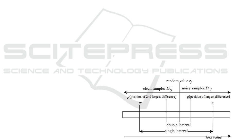
this paper constructs the double interval p,q, which

is based on the single interval m,n, as shown in

Figure 1.p,q is a subinterval of m,n, which means

mpqn. p is the position of the sample with

the second largest difference between adjacent

samples in the ordered loss value array in the entire

ordered array, q is the position of the sample with the

largest difference between adjacent samples in the

ordered loss value array in the entire ordered array. j

represents any classification experiment.

Figure 1: Schematic diagram of random threshold data

division in the double interval.

Because the loss value of the noise sample is

relatively large, the difference in the loss value

between different noise samples is also relatively

large. In order to avoid the maximum and second-

largest value of 𝑑



from being concentrated on

samples with larger loss values, this paper sets a new

size strategy, which is regarded as the value of 𝑑



larger than 𝑑



when 𝑑



2𝑑



.Through this

Filtered Weighted Correction Training Method for Data with Noise Label

179

constraint, the reliable values of p and q are restricted,

and the algorithm flow is shown as follows.

Algorithm 1: getPQ.

The experimental results of a single sample

classification may be accidental, leading to errors.

Therefore, it is more reliable to construct different

data division combinations by randomly extracting

thresholds multiple times in the interval, and the

intersection of them is more reliable. After N random

selections in the interval m,n, a total of N sets of

data divisions are obtained, which can be expressed

as Equation 1, where 𝐷𝑐



and 𝐷𝑛



are arrays of

indefinite length.

〈

𝐷𝑐



,𝐷𝑛





⋯



𝐷𝑐



,𝐷𝑛



〉

(1)

Consensus voting and majority voting are two

commonly used strategies in ensemble learning. The

main difference lies in the strength of consensus. In

the confidence method, voting can be regarded as the

matching degree between the predicted label and the

actual label. In this method, voting refers to the

number of times that the sample 𝑑



appears in the 𝐷𝑐



data set in 𝐷. Majority voting refers to the number of

times that 𝑑



appears in the 𝐷𝑐



data set in N data

division groups, and the count is greater than the set

threshold. See Formula 2. When 1c2, count

can represent the majority. If you want a more

detailed definition of the majority, you can set it by

adjusting the value of c. In particular, when c=

1,count = N, it represents the consensus vote.

𝑐𝑜𝑢𝑛𝑡 

𝑁

𝑐

(2)

Consistent voting is equivalent to taking the

intersection of each division result. This screening

method will cause the voting result to be excessively

dependent on each data division situation. It is more

sensitive to any abnormal classification and has poor

robustness. The traditional majority voting method,

that is, the count counting method when c=2, will

increase the unreliability of the final voting result.

Therefore, this paper adjusts the value of c to achieve

the purpose of mixed consensus voting and majority

voting. In the course of the experiment, c is assigned

a value of 1.25, which is based on the same voting

situation of 80% and above. Increase the reliability of

voting results by reducing the influence of abnormal

samples on the classification situation.

In summary, the complete noise tag filtering

algorithm (RTD, Random Threshold in Double

Interval) based on the random threshold in the double

interval can be summarized as the steps.

Algorithm 2: RTD algorithm.

2.2 Weighted Correction Training

Method

The network model tends to learn simple samples in

the early stage of training, and learns the more

difficult noise samples in the later stage of training (J.

Huang et al. 2019). Therefore, the model can still

DeLTA 2021 - 2nd International Conference on Deep Learning Theory and Applications

180

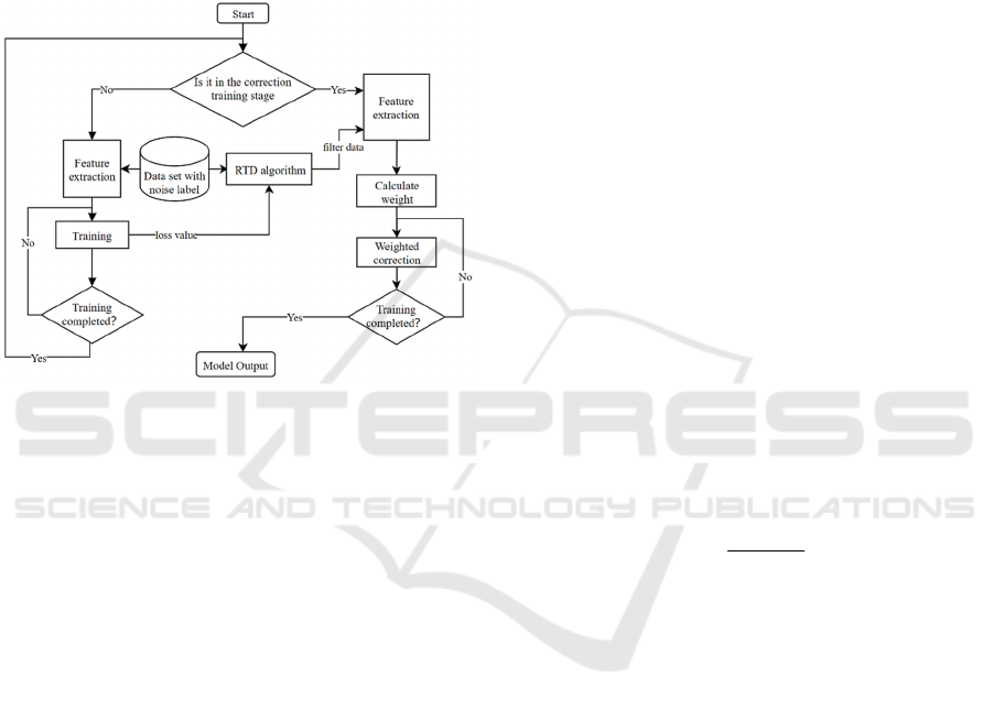
learn clean sample features through early training on

the basis of noisy data. The reason for the decrease in

model accuracy is often the over-learning of noise

samples in the later stage of training. Therefore, this

article adds an early stopping mechanism to the

network model training to reduce the impact of noise

samples in the later stage of training by reducing the

number of rounds, and then use the filtered data for

weighted correction training to guide the fine-tuning

of the trained model.

Figure 2: Flow chart of weighted correction training method

after filtering.

Let W be a weighted vector, as shown in Equation

3, where w



is the weighted value of the i-th tag

category.

𝑊=

〈

𝑤



,𝑤



,𝑤



⋯,𝑤



〉

(3)

Assuming that the sample prediction vector is Y,

the loss value of different types of samples can be

modified by the dot product operation between the

weighting vector W and the sample prediction vector

Y, so that the correction network generates different

loss values for different label categories. The loss

value plays a role in guiding the adjustment of various

parameters of the neural network during the back

propagation process. When misclassification occurs,

when the original loss value is the same, the label

category with a larger weight value has a greater

impact on the adjustment of each parameter of the

neural network than the label category with a smaller

weight value. This way of constructing the loss value

can encourage the model to learn more sample

characteristics of the label category with a large

weight value. In the calibration training stage, this

way of controlling the optimization direction of the

model can make the model pay more attention to the

samples that perform poorly during the training

process.

Assuming that the sample prediction vector Y is

Equation 4, the situation after weighting calculation

is shown in Equation 5, which is adding category

weight to the corresponding label category.

𝑌=

〈

𝑦



,𝑦



,𝑦



⋯,𝑦



〉

(4)

𝑌



〈

𝑤



𝑦



,𝑤



𝑦



,𝑤



𝑦



⋯,𝑤



𝑦



〉

(5)

Since the filtered data is used in the weighted

correction training stage, a loss function with strong

fitting ability, such as a cross-entropy loss function,

should be used. At this time, the process of

calculating the loss value can be expressed as

Equation 6, if and only if 𝑦



is 1, the loss value is 𝑤



times the original value.

𝑙𝑜𝑠𝑠 = 𝑦





log𝑦







=𝑤



𝑦



log𝑦





(6)

From the above analysis, it can be known that the

weight vector W is related to the model performance

after the preliminary training, that is, before the

correction training. Assuming that the accuracy of

each label category before correction training is

vector A, where the classification accuracy of the i-th

label category is 𝑎𝑐𝑐



, then the weighted value 𝑤



the i-th label category can be expressed as Equation

𝑤



𝑡

1 + 𝑎𝑐𝑐



(7)

Among them, the parameter t is responsible for the

adjustment of the weighted value of each label

category. The recommended value is 2,4. Too small

value makes the samples indistinguishable, and too

large value will cause the model learn too much from

the samples under the label category with a larger

weight. Over-optimization reduces overall

performance. In particular, when the sample accuracy

rate is 0, such as when the sample data of this category

does not exist in the training process, etc., the

weighted value 𝑤



still has a mathematical meaning

under Formula 7. When the sample accuracy rate is 1,

if the predicted value of the sample of this category is

100% correct, if the value of t is 2 at this time, the

corresponding 𝑤



value is 1, that is, no weighting

operation is performed.

In summary, the overall process of the filtered

weighted correction training method can be shown as

Figure 2.

Filtered Weighted Correction Training Method for Data with Noise Label

181

3 RESULTS AND ANALYSIS

In order to verify the effectiveness of the WCF

training method, the current commonly used data

preprocessing methods are selected for comparison,

including a random threshold in a single interval, a

fixed threshold, and the RTD tag noise filtering

algorithm proposed in this paper. The mircoF1 of the

model is used as a measurement index, and each

experiment is repeated 5 times with the average value

as the final effect to reduce chance.

The CIFAR10 data set was randomly modified

with label values from 10% to 60% to construct noise

data to explore the performance of the WCF training

method under different noise ratios r. In the selected

label filtering algorithm, the first interval is set to

[0.4, 0.8], the loss function is the cross-entropy loss

function, and the noise label filtering data is the first

10 rounds of training results, that is, the 10 division

results are used for ensemble learning.

Use the three-layer convolutional neural network

(called CNN3), VGG16 and ResNet50 to conduct

experiments to explore the performance of the WCF

algorithm in different depths and different scales of

network models.

Use the precision rate P defined by Equation 8 and

the recall rate R defined by Equation 9 to measure the

performance of the RTD noise filtering algorithm.

𝑃=

TP + FP

(8)

𝑅=

TP + FN

(9)

Where TP represents the number of clean samples

classified as clean samples, FP represents the number

of noise samples classified as clean samples, FN

represents the number of clean samples classified as

noise samples, and TN represents the number of noise

samples classified as noise samples Number.

3.1 Effectiveness Analysis of Noise

Filtering Algorithm

The experiment in this section mainly explores the

performance of the RTD algorithm relative to the

random threshold division method in the one-fold

interval and the fixed threshold division method for

clean sample extraction. This section discusses the

effects of different methods from the two perspectives

of precision and recall of the extracted clean samples.

In addition, considering that the noise rate of the data

set is unknown in actual production and life, it is also

meaningful to integrate the performance of the

method under different noise rates. The experimental

models all use ResNet50, and the experimental results

are recorded in Table 1.

It can be seen from Table 1 that the average effect

of the RTD algorithm is the best. Compared with the

filtering method of a single interval random

threshold, the RTD algorithm not only improves the

accuracy rate by nearly 1%, but also improves the

recall rate by 5%. This means that under the same

Table 1: The performance of different noise filtering algorithms under different noise rates.

noise

rate

RTD(our method)

random threshold in

the one-fold interval

fixed threshold

0.4

fixed threshold

0.6

fixed threshold

0.8

P R P R P R P R P R

0.1 0.998 0.626 0.998 0.418 0.994 0.033 0.999 0.440 0.995 0.816

0.2 0.989 0.678 0.992 0.429 0.988 0.052 0.993 0.511 0.965 0.899

0.3 0.965 0.675 0.963 0.526 0.961 0.096 0.971 0.620 0.879 0.942

0.4 0.920 0.665 0.909 0.548 0.899 0.142 0.900 0.678 0.764 0.950

0.5 0.823 0.516 0.803 0.574 0.791 0.178 0.786 0.696 0.650 0.946

0.6 0.633 0.475 0.616 0.537 0.606 0.171 0.605 0.639 0.510 0.913

0.7 0.428 0.465 0.418 0.431 0.406 0.157 0.424 0.585 0.373 0.873

0.8 0.266 0.329 0.265 0.474 0.271 0.187 0.264 0.518 0.236 0.794

0.9 0.103 0.380 0.101 0.381 0.097 0.167 0.102 0.434 0.101 0.716

Average 0.681 0.534 0.674 0.480 0.668 0.131 0.672 0.569 0.608 0.872

DeLTA 2021 - 2nd International Conference on Deep Learning Theory and Applications

182

accuracy rate, the RTD algorithm can identify more

clean samples. Compared with other fixed threshold

methods, the RTD algorithm can increase the average

accuracy rate by 1.5% to 7.3%.

When the noise rate is low, that is, r≤0.3, the

filtering method with a single threshold of 0.6 has a

higher recognition accuracy for clean samples, but the

performance is not much different from other

methods. This is caused by the large difference in loss

between clean samples and noise samples at low

noise rates. Large numerical differences lead to

strong distinguishability, which ultimately leads to a

higher overall level of accuracy at low noise rates.

Under the same circumstances, the RTD method can

increase the recall rate while ensuring high accuracy,

and screen out more samples, which is more

conducive to the retention of clean samples.

When the noise rate is high, that is, r≥0.8, the

accuracy of each method is not much different. Except

for the filtering method with a single threshold of 0.8,

the difference in accuracy of other methods is within

1%. This is because when the threshold is set to a fixed

value of 0.8, most of the samples will be retained, and

the number of retained samples far exceeds the actual

number of clean samples. Therefore, the filtered data

contains a lot of noise data, which leads to a decrease

in accuracy. In real life, the data set with too high noise

rate should be cleaned first, and a batch of obvious

noise samples should be deleted according to the data

logic to reduce the noise rate before putting it into noise

label filtering.

When the noise rate is 0.4≤r≤0.7, the RTD

algorithm has a 0.4%~17.3% improvement in

accuracy compared with other methods. In particular,

compared with the one-fold interval random

threshold method, the accuracy is improved by

1.1%~2%. This is because the setting of the double

interval reduces the range of possible values of the

random threshold, so that under the unknown noise

rate, the proportion of clean samples is reasonably

estimated to increase, and the probability of the

effective threshold is increased to improve the

recognition accuracy.

3.2 Effectiveness Analysis of the

Weighted Correction Training

Method after Filtering

In this section, the experimental results of the WCF

training method proposed in this paper and the

common method preprocessed by the label noise

filtering algorithm under different noise rates and

different model scales are recorded in Table 2.

Table 2: F1 values of WCF combined optimization schemes under different models under different noise rates.

noise rate 0.1 0.2 0.3 0.4 0.5 0.6

CNN3

38.92% 33.20% 30.40% 28.57% 26.47% 22.65%

CNN3+WCF(Method of this article)

40.95% 34.77% 32.42% 31.67% 30.49% 29.49%

CNN3+RTD

33.56% 32.12% 31.66% 30.87% 29.35% 27.57%

CNN3+ fixed threshold in the one-fold interval

30.46% 30.63% 28.60% 27.15% 24.49% 20.97%

CNN3+ fixed threshold 0.6

33.25% 32.27% 28.69% 27.68% 25.36% 24.03%

VGG16

77.71% 67.84% 60.16% 49.82% 39.46% 28.81%

VGG16 +WCF(Method of this article)

84.24% 71.23% 62.95% 52.30% 41.82% 29.93%

VGG16+RTD

79.38% 68.23% 61.14% 50.56% 38.16% 27.70%

VGG16+ fixed threshold in the one-fold interval

77.24% 65.45% 52.47% 47.06% 37.54% 27.37%

VGG16+ fixed threshold 0.6

77.95% 62.54% 48.51% 46.26% 35.85% 29.08%

ResNet50

77.98% 60.88% 54.07% 46.74% 36.36% 26.02%

ResNet50 +WCF(Method of this article)

80.53% 62.41% 56.70% 49.80% 39.67% 28.89%

ResNet50+RTD

79.02% 61.56% 54.71% 46.44% 37.69% 26.49%

ResNet50+ fixed threshold in the one-fold interval

75.05% 61.15% 53.22% 41.49% 34.65% 25.59%

ResNet50+ fixed threshold 0.6

75.61% 60.79% 52.96% 44.32% 35.42% 26.43%

Filtered Weighted Correction Training Method for Data with Noise Label

183

It can be seen from Table 2 that the WCF method

proposed in this article performs best at any noise

rate. Compared with other methods, the F1 value of

the model is improved by 0.76%~14.44% under

different noise rates and different network depths.

The model obtained by the RTD preprocessing

data is better than other methods. Compared with

other filtering methods, the RTD method blurs the

threshold boundary while reasonably narrowing the

threshold value range and increasing the accuracy of

the division. The experimental results demonstrate

the effectiveness of the filtering algorithm used in the

WCF method.

Using filtering algorithms to preprocess the data

does not necessarily increase the model F1 value

significantly. This is because the filtering algorithm

reduces the size of the data set while improving the

accuracy of the data set. While filtering out noise

samples, a large number of clean samples do not enter

the training process. The WCF method retains the

initial training process to avoid the decrease in model

accuracy caused by the reduction of sample size. In

addition, increasing the proportion of clean samples

can achieve almost the same effect as using the

original data, but the reduction in the amount of data

can significantly reduce the time and space loss of

training the model.

Compared with single training, the WCF method

can increase the model F1 value by 1.12%~6.84%.

The effect is better under low noise, deep networks,

and the best effect is for simple networks under high

noise conditions. In VGG16, as the noise rate

increases, the gain between the WCF optimization

method and the original training method gradually

decreases. The main reason is that the deeper network

learns the model more thoroughly, so the noise in the

filtered sample is deeper in the weighted correction

process.

In summary, the WCF training method has better

model performance than single training and data pre-

processing before training.

4 CONCLUSIONS

This paper proposes a filtered weighted correction

training method for the data set with noise label. The

accuracy of the model is improved by adding a

weighted correction stage after the model training.

The data used in the correction training is filtered by

a random threshold algorithm in the double interval

sample. The proposed method performs well in

models of different depths.

ACKNOWLEDGEMENTS

This work is funded by the Open Fund Project of

Science and Technology on Communication

Networks Laboratory (Grand No. HHX21641X003).

REFERENCES

Algan G., Ulusoy I., (2019). Image classification with deep

learning in the presence of noisy labels: a survey.

Retrieved from https://arxiv.org/abs/1912.05170.

Song H., Kim M., Park D., et al. (2020). Learning from

Noisy Labels with Deep Neural Networks: A Survey.

Retrieved from https://arxiv.org/abs/2007.08199.

Nicholson B., Sheng S. V., Zhang J., (2015). Label noise

correction and application in crowdsourcing. In Quebec

City, 2015 IEEE International Conference on Image

Processing (ICIP), pp. 1458-1462.

Han B., Yao Q., Yu X., (2018). Co-teaching: Robust

training of deep neural networks with extremely noisy

labels.In Montréal, Canada, NeurIPS.

Zhang Z., Sabunc M., (2018). Generalized cross entropy

loss for training deep neural networks with noisy labels.

In Montréal, Canada, NeurIPS.

Wang Y., Ma X., Chen Z., et al. (2019). Symmetric cross

entropy for robust learning with noisy label. In IEEE

International Conference on Computer Vision.

Zhang Z. Z., Jiang GX & Wang J. W., (2020). Label noise

filtering method based on local probability. Journal of

Computer Applications, 1-9.

Sluban, B., Gamberger, D. & Lavrač, N. (2014). Ensemble-

based noise detection: noise ranking and visual

performance evaluation. Data Min Knowl Disc 28, 265-

303.

Y. Wei, C. Gong, S. Chen, T. Liu, J. Yang & D. Tao, (2020).

Harnessing Side Information for Classification Under

Label Noise. IEEE Transactions on Neural Networks

and Learning Systems, vol. 31, no. 9, pp. 3178-3192.

Frénay B., Verleysen M. (2014). Classification in the

presence of label noise: a survey. IEEE transactions on

neural networks and learning systems, 2014, 25(5):

845-869.

Chen Q. Q., Wang W. J., Jiang G. X., (2019). Label noise

filtering based on the data distribution. Journal of

Tsinghua University (Science and Technology), 59(4):

262-269.

Lei S. H., Zhang H., Wang K., et al. (2019). How Training

Data Affect the Accuracy and Robustness of Neural

Networks for Image Classification. In ICLR 2019.

J. Huang, L. Qu, R. Jia & B. Zhao, (2019) O2U-Net: A

Simple Noisy Label Detection Approach for Deep

Neural Networks. In Seoul, Korea (South), IEEE/CVF

International Conference on Computer Vision (ICCV),

pp. 3325-3333.

Zhang C. Y., Samy Bengio, Moritz Hardt et al. (2017).

Understanding deep learning requires rethinking

generalization. In ICLR 2017.

DeLTA 2021 - 2nd International Conference on Deep Learning Theory and Applications

184