FROM DIOID ALGEBRA TO P-TIME EVENT GRAPHS

Mohamed Khalid DIDI ALAOUI

Philippe DECLERCK

LISA FRE 2656 CNRS

ISTIA, 62, Av Notre Dame du Lac, 49000 Angers, France

Keywords:

(min,max,+) functions, cycle-time vector, ﬁxed point, P-time event graphs.

Abstract:

The (max,+) algebra is usually used to model Timed event graph. In this paper, we show that P-time event

graphs which extend Timed event graph, can be modelled using maximum, minimum and addition operations.

The result is a new model called interval descriptor system where the time evolution is not strictly deterministic

but belongs to intervals. The cycle-time vector allows us to to check its correct behaviour and to verify the

existence of a state trajectory. Particularly, it detects the presence of token-deads which can generate a dead-

lock.

1 INTRODUCTION

Discrete Event Dynamic Systems can represent a

great number of processes characterized as being con-

current, asynchronous, distributed or parallel, such as

ﬂexible manufacturing systems, multiprocessor sys-

tems or transportation networks. In such systems

the behaviour depends on complex interactions of the

timing of various discrete events. The topical alge-

bra is an important ﬁeld of mathematical and anal-

ysis techniques of these models. The (max,+) al-

gebra makes it possible to analyse the Timed Event

Graphs and many results are available like spectral

theory and control synthesis. In this paper, a new class

of systems is studied for which the time evolution is

not strictly deterministic but belongs to intervals. At

each step, the lower and upper bounds depends on the

maximization, minimization and the addition opera-

tions simultaneously. The symbol ⊕ stands for the

maximum operation while ∧ corresponds to the min-

imum operation. The operation ⊕ has the neutral el-

ement ε = −∞ whereas ∧ has the neutral element

T = +∞. The notations ⊗ and ¯ corresponds to the

usual addition with the following convention: T ⊗ε =

ε and T ¯ ε = T. The expression a ⊗ b and a ¯ b are

identical if at least either a or b is a ﬁnite scalar.

We propose to analyse the following implicit model

called interval descriptor system. The evolution of the

system is described by the following equations where

and f

−

are (min, max, +) functions. The interpre-

tation of each variable is as follows: like the ”dater”

type in (max,+) algebra, each variable x

(k) repre-

sents the date of the kth ﬁring of transition x











x(k) = x(k) ∧ f

(x(k), ..., x(k − m), u(k)

, ..., u(k − m))

x(k) = x(k) ⊕ f

−

(x(k), ..., x(k − m), u(k)

, ..., u(k − m))

with x(k) = ² for k ≤ 0

(1)

The vector u is the input and m is the horizon. We

can also introduce the output y by y(k) = C ⊗ x(k).

To simplify the writing, the matrix C will be chosen

to make a direct correspondence between some com-

ponent of x

(k) and a component of output y

(k) in a

natural manner. Consequently, some columns can be

null but each row contains only one element e = 0

and ε elsewhere. This equality will not be used in this

paper. The functions f

() and f

−

() represent respec-

tively an upper and lower bound of x whose trajectory

is between these bounds. Particularly, if the lower

bound deﬁned by f

−

is a (max, +) function and the

upper bound is inﬁnite, the classical (max, +) systems

can be obtained after some classical manipulations.

In this paper, we give in a ﬁrst part some preliminar-

ies and important ﬁxed-point theorems. We then in-

troduce a class of interval descriptor system and show

that P-time event graphs can be modelled under this

form. Finally, we analyze the correct behaviour of p-

330

Khalid DIDI ALAOUI M. and DECLERCK P. (2004).

FROM DIOID ALGEBRA TO P-TIME EVENT GRAPHS.

In Proceedings of the First International Conference on Informatics in Control, Automation and Robotics, pages 332-337

DOI: 10.5220/0001137403320337

 SciTePress

time event graphs and particulary the synchronization

of transitions.

2 PRELIMINARIES

The partial order denoted 6 is deﬁned as follows: x 6

y ⇐⇒ x ⊕ y = y ⇐⇒ x ∧ y = x ⇐⇒ x

6 y

, for i

from 1 to n in <

. Notation x < y means that x 6 y

and x 6= y.

Deﬁnition 2.1 A dioid D is complete if it is closed

for inﬁnite sums and the distributivity of the multipli-

cation with respect to addition extends to inﬁnite sums

: (∀ c ∈ D ) (∀ A ⊆ D) c ⊗ (

x∈A

x) =

x∈A

c ⊗ x

For example,

max

= (< ∪ {−∞} ∪ {+∞}, ⊕, ⊗)

is complete.

The set of n.n matrices with entries in a complete

dioid D endowed with the two operations ⊕ and ⊗

is also a complete dioid which is noted D

n.n

. The

elements of the matrices in the (max, +) expressions

(respectively (min, +) expressions) are either ﬁnite or

ε ((respectively T ). We can deal with nonsquare ma-

trices if we complete by rows or columns with entries

equals to ε ( respectively T). The different operations

operate as in the usual algebra: The notation ¯ refers

to the multiplication of two matrices in which the ∧

operation is used instead of ⊕.

(A ⊕ B)

= A

⊕ B

(A ∧ B)

= A

∧ B

(A ⊗ B)

k=1

⊗ B

(A ¯ B)

k=1

¯ B

In (⊕, ⊗) algebra, Kleene’s star is deﬁned by:

∗

+∞

i=0

. Respectively, in (∧, ¯) algebra,

Kleene’s star is deﬁned by: A

∗

+∞

i=0

Noted as G(A), an induced graph of a square ma-

trix A is deduced from this matrix by associating

- a node i to the column i and line i

- an arc from the node j towards the node i if A

ε.

Theorem 2.2 (F. Baccelli and Quadrat, 1992)

Given A and B in a complete dioid and consider

the equation x = A ⊗ x ⊕ B and the inequality

x > A ⊗ x ⊕ B . Then, for these expressions :

∗

⊗ B is the least solution ; every solution x ver-

iﬁes x = A

∗

⊗ x ; T is the greatest solution of the

inequality.

Theorem 2.3 Given A and B in a complete dioid

and consider the equation x = A ¯ x ∧ B and the

inequality x 6 A¯x∧B . Then, for these expressions

: A

∗

¯ B is the greatest solution ; every solution x

veriﬁes x = A

∗

¯ x ; ε is the least solution of the

inequality.

The left ⊗ residuation of b by a is deﬁned by:

a\b = max{x ∈ D such that a ⊗ x 6 b}. Respec-

tively, in (∧, ¯) algebra, the left ¯ residuation of b

by a is deﬁned by: a\

b = min{x ∈ D such that

a ¯ x > b}.

Given A and B two matrices in a complete dioid,

the residuation of B ( dimensions n.q ) by A (dimen-

sions n.p) is clearly expressed in the other dioid:

A\B = (−A)

¯ B and A\

B = (−A)

⊗ B with

t: transpose.

Lemma 2.4 part1 (F. Baccelli and Quadrat, 1992) We

have the following equivalences: x ≥ ax ⇔ x =

∗

x ⇔ x ≤ a \ x ⇔ x = a

∗

\ x

3 INTERVAL DESCRIPTOR

SYSTEM AND COMPATIBILITY

3.1 Cycle time and compatibility

Now, we introduce the deﬁnitions of cycle time,

eigen-vector, eigen-value and ultimately afﬁne

regime (Cheng and Zheng, 2002)(Gaubert and Gu-

nawardena, 1998). These notions are relevant to the

(min, max, +) functions but not always to the topical

functions. Some connections can be established

between these concepts. Addition + is deﬁned by:

∀λ ∈ <, ∀x ∈ <

, λ + x = (λ + x

, ..., λ + x

)

(t:

transpose)

Deﬁnition 3.1 A min-max function of type (n, 1)

is any function f : <

→ <

, which can be written

as a term in the following grammar:

f = x

, x

, · · · x

| f + a | f ∧ f | f ⊕ f where a is

an arbitrary real number (a ∈ <)

We consider dynamics of the form:

x(k) = f(x(k − 1)) , ∀k > 1

x(0) = ξ ∈ <

where f is a (min, max, +) function of type (n, n)

→ <

. The set of min − max function of type

(n, m) is noticed D

∗

(n, m).

Deﬁnition 3.2 The cycle time vector is deﬁned by

χ(f) = lim

k→∞

x(k)/k if it exists. It does not depend

on ξ.

Deﬁnition 3.3 An eigen-vector x and its associated

eigen-value λ ∈ <, if they exists, verify f(x) = λ+x

Deﬁnition 3.4 The pair (η, v) ∈ (<

)

is an ulti-

mately afﬁne regime of f if there exists an integer K

such that ∀k > K , f(v + kη) = v + (k + 1)η.

Corollary 3.5 (J. Cochet-Terrasson and Gunawar-

dena, 1999) Any function in D

∗

has a cycle time.

FROM DIOID ALGEBRA TO P-TIME EVENT GRAPHS

331

Moreover, χ(f)= η, for all ultimately regimes (η, v)

∈ (<

)

of f.

In the following theorems, the notion of cycle time

which always exists in D

∗

makes it possible to check

the existence of a solution of different inequalities and

equalities.

Theorem 3.6 (Gaubert and Gunawardena, 1998)

Let f ∈ D

∗

. The two following conditions are equiv-

alent:

(i) It exists a ﬁnite x such that x 6 f(x)

(ii) χ(f) > 0

Theorem 3.7 Let f ∈ D

∗

. The two following con-

ditions are equivalent:

(i) It exists a ﬁnite x such that x > f(x)

(ii) χ(f) 6 0

From the two previous theorems 3.6 and 3.7, we

deduce directly the following result.

Theorem 3.8 Let f ∈ D

∗

. The two following con-

ditions are equivalent:

(i) It exists a ﬁnite x such that x = f(x)

(ii) χ(f) = 0

A set S of min-max functions is rectangular if for

all G, G

∈ S, and for all i = 1, ..., n the function

obtained by replacing the i-th component of G by the

i-th component of G

belongs to S. We denote by

rec(S) the rectangular closure of a set S, which is ﬁ-

nite when S is ﬁnite. Let S, T be rectangular max and

min representations, respectively, of f. Since min-

max functions are monotone,

g∈T

χ(g) 6 χ(f) 6

h∈S

χ(h)

The duality conjecture states that the extreme sides

coincide. It was proved in (Gaubert and Gunawar-

dena, 1998)

χ(f) =

h∈S

χ(h) =

g∈T

χ(g)

Theorem 3.9 (J. Cochet-Terrasson and Gunawar-

dena, 1999) Let f ∈ D

∗

and suppose that

S, T ∈ D

∗

are rectangular and, respectively, a max-

representation and a min-representation of f . The fol-

lowing conditions are equivalent.

1. f has a ﬁxed point with f(x) = x + h.

h²S

χ(h) = h

g²T

χ(g) = h

Remark : The theorem 3.8 can be considered as a

corollary of the theorem 3.9 when h equals 0.

3.2 Generalized Upper Bound

Constraint and Lower Bound

Constraint forms.

In the aim of reducing the size of the expressions, the

system 1 can classically be transformed in reduced

form by increasing the vector state. With an abuse

of notation, we keep the same notation for x, f

−

and

to alleviate the notation. From the system 1, we

deduce:

x(k) 6 f

(x(k), x(k − 1), u(k))

x(k) > f

−

(x(k), x(k − 1), u(k))

As f

and f

−

are (min, max, +) functions, the

above form is more general that the ”UBC” (Upper

Bound Constraint) where f

is a max-only function

(see (Walkup and Borriello, 1998) for more details).

We can call the above forms respectively, ”GUBC”

(Generalized Upper Bound Constraint) and ”GLBC”

(Generalized Lower Bound Constraint). As the above

theorems 3.6, 3.7 and 3.8 can only be applied to the

forms x 6 f(x) , x > f (x) or x = f(x) where

f ∈ D

∗

, we must consider special cases. As the type

of the system 1 is deﬁned by the types of the functions

and f

−

, we can characterize the model by the cou-

ple (type of f

−

, type of f

). The type ((min, max,

+), (min, max, +)) represents the more general case

for the system 1 . Under the assumption of the exis-

tence of a solution, they deﬁne corresponding classes

of compatible interval descriptor systems. In the next

sections, we will only consider the ((max, +), (min,

+)) type and show that the p-time event graphs can be

modelled under this form.

3.3 ((max, +), (min, +)) type

We consider the following system 3.3 of ((max, +),

(min, +)) type :

−

(z(k)) =

i=0

−

⊗ x(k − i) ⊕ B

−

⊗ u(k) and

(z(k)) =

i=0

¯ x(k − i) ∧ B

¯ u(k). (3.3)

Theorem 3.10 The system 3.3 is compatible in the

horizon [k − 1, k] if and only if the cycle time of the

following function g

is greater than or equals zero.

(z(k) =





(z(k)) ∧ A

−

\ x(k)

−

\ x(k)

−

\ x(k)





with z(k) =

x(k)

x(k − 1)

u(k)

Theorem 3.11 The system 3.3 is compatible in the

horizon [k − 1, k] if and only if the cycle time of the

following function g

−

is lower than or equals zero.

−

(z(k) =





−

(z(k)) ⊕ A

x(k)





Corollary 3.12 If the system 3.3 is compatible in

the horizon [k − 1, k], then the following are equiva-

lent.

1. The cycle time of the following function g

greater than or equals zero.

ICINCO 2004 - SIGNAL PROCESSING, SYSTEMS MODELING AND CONTROL

332

2. the cycle time of the following function g

−

lower than or equals zero.

Finally, the ﬁnal inequality set presents the form

−

(z(k)) ≤ z(k) ≤ g

(z(k)). The system of ((max,

+), (min, +)) type is reduced to a (−∞, (min, +))

(respectively ((max, +), +∞))) type and can be an-

alyzed by the theorem 3.10 (respectively the theorem

3.11). If the cycle time veriﬁes the corresponding

condition of existence, it describes a compatible in-

terval descriptor system.

We propose now a generalization of the preceding

theorems on a wider horizon [k, k + h].

Theorem 3.13 The system 3.3 is compatible in the

horizon [k, k + h] if and only if the cycle time of the

function g

(z(k)) is greater than or equals zero.

z(k) =







x(k)

x(k + h − 1)

x(k + h)

u(k)

u(k + h − 1)

u(k + h)







, g

(z(k)) =







(x(k), x(k − 1), u(k))

(x(k + h − 1), x(k + h − 2), u(k + h − 1))

(x(k + h), x(k + h − 1), u(k + h))







∧ M

\ z(k) ∧ z(k + 1)

with M =







−

· · · T

. A

−

T · · · A

−







, M







−

T · · · T

. B

−

T · · · B

−







and M

= M

= T

Proof

For 0 ≤ j ≤ h we have :

(

x(k + j) ≤ f

(x(k + j), x(k + j − 1), u(k + j))

x(k + j − 1) ≤ x(k + j)

u(k + j − 1) ≤ u(k + j)

and A

−

⊗ x(k + j) ⊕ A

−

⊗ x(k + j − 1) ⊕ B

−

⊗

u(k + j) ≤ x(k + j)

we use the lemma 2.4, we arrive to :

⇐⇒







x(k + j) ≤ A

−

\ x(k + j)

x(k + j − 1) ≤ A

−

\ x(k + j)

u(k + j) ≤ B

−

\ x(k + j)

let x(k) = ² for k ≤ 0

A concatenation of the two last systems gives the fol-

lowing form : ∀ 0 ≤ j ≤ h











x(k + j) ≤

(x(k + j), x(k + j − 1), u(k + j))

∧A

−

\ x(k + j)∧

−

\ x(k + j + 1) ∧ x(k + j + 1)

u(k + j) ≤ B

−

\ x(k + j) ∧ u(k + j + 1)

and











x(k + h)

≤ f

(x(k + h), x(k + h − 1), u(k + h))

∧A

−

\ x(k + h)

u(k + h) ≤ B

−

\ x(k + h)

Lastly, the above system can be reduced to the

following form where the function g

is described in

the body of the theorem.

z(k) ≤ g

(z(k))

4 P-TIME PETRI NETS AND

ACCEPTABLE FUNCTIONING

4.1 Modelling

The p-time Petri nets make it possible to model the

discrete event dynamic systems with time constraints

of stay of the tokens inside the places. We associate

for each place a temporal interval.

Deﬁnition 4.1 (p-time Petri nets) The formal deﬁ-

nition of p-Time PN is given by a pair < R, IS >

where R is a marked Petri nets

IS : P −→ (Q

∪ {0}) × (Q

∪ {∞})

−→ IS

= [a

, b

] with 0 ≤ a

≤ b

is the static interval of residence time or dura-

tion of a token in place p

. The value a

is the min-

imum residence duration that the token must stay in

the place p

. Before this duration, the token is in state

of unavailability to ﬁring the transition t

. The value

is a maximum residence duration after which the

token must thus leave the place p

. If not, the sys-

tem is found in a token-dead state. We conclude that

the token is available to ﬁring the transition t

in the

interval time [a

, b

We will express the interval of shooting of each

transition from the system which will guarantee an

acceptable functioning. The assumption of function-

ing FIFO of the transition x

guarantees the condition

of non overtaking of the tokens between them. We

consider S the set of all input places to transition x

FROM DIOID ALGEBRA TO P-TIME EVENT GRAPHS

333

For the p-time PNs, the evolution is described by the

following inequations :

(k) ≥

j∈S

(k − m

) + a

)

with a

the lower bound of an upstream place of x

and m the number of tokens present in an upstream

place of x

and

(k) ≤

j∈S

(k − m

) + b

)

with b

the upper bound of an upstream place of x

In this part, we study p-time event graphs which is

an example of ((max, +), (min, +)) type of interval

descriptor system.

Remarks : - If one of the m tokens of a place p

dies

before ﬁring transition x

, this death is translated

in the state equations. The new model becomes :

j∈S−{p

}

(k − m

) + a

) ⊕ (x

(k − m

− 1) +

) ≤ x

(k) ≤

j∈S−{p

}

(k−m

)+b

)∧(x

(k−

− 1) + b

)

- If we divide up each place which contains m to-

kens in m places, with one token by place, we can

obtain the equations on a shorter horizon. Only the

upstream place of x

has temporization [a, b]. For the

others, they have all the null time interval [0, 0].

4.2 Analysis of transition

synchronization in an horizon

The Petri nets make it possible to analyze several be-

havioral or structural properties related to the systems

which they model. We consider one of these behav-

ioral properties, the liveness which ensures the system

not to reach a state of blocking. This property depends

on initial marking. A state of blocking in PNs occurs

when we reach a marking which does not allow the

ﬁring of any transition. Now we give the formal deﬁ-

nition of liveness.

Deﬁnition 4.2 (liveness of a transition) A

transition x

is live for an initial marking M

if,

for any marking M

accessible since M

there is a

sequence of ﬁring S starting from M

which includes

the transition x

Deﬁnition 4.3 (liveness of a petri net) For a given

initial marking, a PN is live if for any accessible

∀ M ∈ E(M

), ∀ p ∈ P, ∃ S Á M

−→ M

and t

∈ S

Classically, one of the methods which allow to

check liveness is analysis by enumeration. This

approach consists in building the coverability graph if

the number of markings is ﬁnished, or in building the

coverability tree if the number of markings is inﬁnite.

For temporal PNs, checking and making study of the

liveness property becomes more difﬁcult since the

latter depends not only on initial marking but also

on the intervals of times related to the graph. It thus

proves that the use of the method by enumeration

is very difﬁcult. Indeed, the passage of a state to

another is related either to the ﬁring of a transition or

to the evolution from time. Thus, a consequence is

combinative explosion of the coverability graph.

As p-time event graphs can be modelled under ((max,

+),(min, +)) interval descriptor system, we propose to

apply the results presented in the part 3 to detect any

non-synchronization of transitions in an horizon. The

following deﬁnition of acceptable functioning on an

horizon will allow us to express easier the approach.

In a practical point of view, the deaths of token

represent the lost of ressources and must naturally be

avoid. Consequently, if we check the acceptable func-

tioning, we guarantee a correct behaviour. Moreover,

we can deduce that the corresponding system is live

on the same horizon. Let us notice that the reverse

is not true: the existence of a non-synchronization

of a transition entails the death of at least one token

but the liveness of the petri net can be ensured by the

other tokens.

Deﬁnition 4.4 (acceptable functioning) We call an

acceptable functioning of a p-time PN any dynamic

evolution of the system without leading to a mark-

dead state or a blocking state.

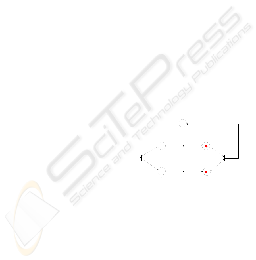
[ a

]

[ a

] [ a

]

[ a

]

[ a

]

Figure 1: a p-time event graph (autonomous case)

Example

We consider the example of the ﬁgure 1 which will

enable us to illustrate our approach. Initially we can

check easily that the logical graph (without taking ac-

count of temporizations) is quite live. By considering

temporizations related to each place, we can note that

in spite of an initial marking which ensures the live-

ness of the logical graph, the temporal graph can be

in a state of total blocking. Showing these behaviours,

several cases can arise while acting on the bounds of

the intervals related to the places.

The ﬁrst step of our approach is to model the system

by recurring state equations in the following form:

ICINCO 2004 - SIGNAL PROCESSING, SYSTEMS MODELING AND CONTROL

334











(k) + a

≤ x

(k) ≤ x

(k) + b

(k − 1) + a

) ⊕ (x

(k − 1) + a

) ≤ x

(k)

≤ (x

(k − 1) + b

) ∧ (x

(k − 1) + b

)

(k) + a

≤ x

(k) ≤ x

(k) + b

(k) + a

≤ x

(k) ≤ x

(k) + b

(2)

The second step consists to divide up the system 2,

and to put it in the form x ≤ f(x). Thus we arrive at

the following system:











(k) ≤ (x

(k) + b

) ∧ (x

(k) − a

)

∧(x

(k) − a

)

(k + 1) ≤ (x

(k + 1) + b

) ∧ (x

(k + 1)

−a

) ∧ (x

(k + 1) − a

)

(k) ≤ (x

(k) − a

) ∧ (x

(k) + b

)

(k + 1) ≤ (x

(k + 1) + b

)

Case 1:

Now we present the ﬁrst case where we ﬁx the

bounds of the intervals as follows : [a

] = [0, 1],

] = [5, 6], [a

] = [0, 1], [a

] = [0, 1] and

] = [3, 4].

We calculate the spectral vector of f, and we apply

the theorem 3.13. We arrive at the following results:

χ(x

(1)) =

χ(x

(1)) =

χ(x

(2)) = −

χ(x

(2)) = −

We notice that χ

(1)

≥ 0 and

(2)

< 0

The system is live for the ﬁrst step (k = 1). It

after loses its tokens (dead tokens) and its liveness

property is not assured any more.

Case 2:

A second case is to consider these intervals such as

]∩ [a

] = ∅. The calculation of the spectral

vector will enable us to show the non-liveness of

the system in this case. We consider the following

temporizations : [a

] = [3, 4], [a

] = [1, 2], [a

] = [6, 7] and [a

] = [4, 5]. We

obtain the following results :

χ(x

(1)) = −

χ(x

(1)) = −

Then, in this case, the synchronization cannot be

make to ﬁring transition x

for the ﬁrst time. The

two tokens will die, the system is in state of blocking

from the beginning because χ

(1)

< 0.

5 CONCLUSION

In this paper, we have introduced a new model, the in-

terval descriptor system based on (min, max, +) func-

tions and we have shown that p-time event graphs can

be modelled in this form. The analysis of the spectral

vector makes it possible to study the correct synchro-

nization of the transitions. We have applied our ap-

proach to an example in section 4. A perspective will

be to specify the token-deads and then to analyse the

complete liveness of the model. We will show that

each token-dead produces a variation in the model

which contains the conditions of its own evolutions.

REFERENCES

Cheng, Y. and Zheng, D.-Z. (2002). On the cycle time of

non-autonomous min-max systems. In IEEE.

F. Baccelli, G. Cohen, G. O. and Quadrat, J. (1992). Syn-

chronization and linearity. An Algebra for Discrete

Event Systems. Wiley, New York.

Gaubert, S. and Gunawardena, J. (1998). the duality the-

orem for min-max functions. In CRAS, t. 326, S

erie

I43-48.

J. Cochet-Terrasson, S. G. and Gunawardena, J. (1999). A

constructive ﬁxed point theorem for min-max func-

tions. In Dynamics and Stability of Systems, Vol. 14

◦

4, 407-433.

Walkup, E. A. and Borriello, G. (1998). A general linear

max-plus solution technique. In Idempotency, pub-

lisher Jeremy Guawardena.

FROM DIOID ALGEBRA TO P-TIME EVENT GRAPHS

335