ITERATIVE LINEAR QUADRATIC REGULATOR DESIGN
FOR NONLINEAR BIOLOGICAL MOVEMENT SYSTEMS
Weiwei Li
Department of Mechanical and Aerospace Engineering, University of California San Diego
9500 Gilman Dr, La Jolla, CA 92093-0411
Emanuel Todorov
Department of Cognitive Science, University of California San Diego
9500 Gilman Dr, La Jolla, CA 92093-0515
Keywords:
ILQR, Optimal control, Nonlinear system.
Abstract:
This paper presents an Iterative Linear Quadratic Regulator (ILQR) method for locally-optimal feedback con-
trol of nonlinear dynamical systems. The method is applied to a musculo-skeletal arm model with 10 state
dimensions and 6 controls, and is used to compute energy-optimal reaching movements. Numerical compar-
isons with three existing methods demonstrate that the new method converges substantially faster and finds
slightly better solutions.
1 INTRODUCTION
Optimal control theory has received a great deal of
attention since the late 1950s, and has found appli-
cations in many fields of science and engineering. It
has also provided the most fruitful general framework
for constructing models of biological movement (Y
et al., 1989; Harris and Wolpert, 1998; Lahdhiri and
Elmaraghy, 1999; Todorov and Jordan, 2002). In the
field of motor control, optimality principles not only
yield accurate descriptions of observed phenomena,
but are well justified a priori. This is because the sen-
sorimotor system is the product of optimization pro-
cesses (i.e. evolution, development, learning, adapta-
tion) which continuously improve behavioral perfor-
mance.
Producing even the simplest movement involves an
enormous amount of information processing. When
we move our hand to a target, there are infinitely many
possible paths and velocity profiles that the multi-
joint arm could take, and furthermore each trajec-
tory can be generated by an infinite variety of muscle
activation patterns (since we have many more mus-
cles than joints). Biomechanical redundancy makes
the motor system very flexible, but at the same time
requires a very well designed controller that can
choose intelligently among the many possible alter-
natives. Optimal control theory provides a principled
approach to this problem – it postulates that the move-
ment patterns being chosen are the ones optimal for
the task at hand.
The majority of existing optimality models in mo-
tor control have been formulated in open-loop. How-
ever, the most remarkable property of biological
movements (in comparison with synthetic ones) is
that they can accomplish complex high-level goals in
the presence of large internal fluctuations, noise, de-
lays, and unpredictable changes in the environment.
This is only possible through an elaborate feedback
control scheme. Indeed, focus has recently shifted
towards stochastic optimal feedback control models.
This approach has already clarified a number of long-
standing issues related to the control of redundant
biomechanical systems (Todorov and Jordan, 2002).
In their present form, however, such models have a
serious limitation – they rely on the Linear-Quadratic-
Gaussian formalism, while in reality biomechanical
systems are strongly non-linear. The goal of the
present paper is to develop a new method, and com-
pare its performance to existing methods (Todorov
and Li, 2003) on a challenging biomechanical control
problem. The new method uses iterative linearization
of the nonlinear system around a nominal trajectory,
and computes a locally optimal feedback control law
via a modified LQR technique. This control law is
then applied to the linearized system, and the result is
used to improve the nominal trajectory incrementally.
It has convergence of quasi-Newton method.
The paper is organized as follows. The new ILQR
method is derived in Section 2. In section 3 we
present a realistic biomechanical model of the human
arm moving in the horizontal plane, as well as two
222
Li W. and Todorov E. (2004).
ITERATIVE LINEAR QUADRATIC REGULATOR DESIGN FOR NONLINEAR BIOLOGICAL MOVEMENT SYSTEMS.
In Proceedings of the First International Conference on Informatics in Control, Automation and Robotics, pages 222-229
DOI: 10.5220/0001143902220229
Copyright
c
 SciTePress

simpler dynamical systems used for numerical com-
parisons. Results of applying the new method are pre-
sented in section 4. Finally, section 5 compares our
method to three existing methods, and demonstrates a
superior rate of convergence.
The notation used here is fairly standard. The trans-
pose of a real matrix A is denoted by A
T
; for a sym-
metric matrix, the standard notation > 0 (≥ 0) is
used to denote positive definite matrix (positive semi-
definite matrix). D
x
f(·) denotes the Jacobian of f(·)
with respect to x.
2 ILQR APPROACH TO
NONLINEAR SYSTEMS
Consider a discrete time nonlinear dynamical system
with state variable x
k
∈ R
n
x
and control u
k
∈ R
n
u
x
k+1
= f(x
k
, u
k
). (1)
The cost function is written in the quadratic form
J
0
=
1
2
(x
N
− x
∗
)
T
Q
f
(x
N
− x
∗
)
+
1
2
N−1
X
k=0
(x
T
k
Qx
k
+ u
T
k
Ru
k
), (2)
where x
N
describes the final state (each movement
lasts N steps), x
∗
is the given target. The state cost-
weighting matrices Q and Q
f
are symmetric positive
semi-definite, the control cost-weighting matrix R is
positive definite. All these matrices are assumed to
have proper dimensions. Note that when the true cost
is not quadratic, we can still use a quadratic approxi-
mation to it around a nominal trajectory.
Our algorithm is iterative. Each iteration starts with
a nominal control sequence u
k
, and a corresponding
nominal trajectory x
k
obtained by applying u
k
to the
dynamical system in open loop. When good initial-
ization is not available, one can use u
k
= 0. The iter-
ation produces an improved sequence u
k
, by lineariz-
ing the system dynamics around u
k
, x
k
and solving a
modified LQR problem. The process is repeated un-
til convergence. Let the deviations from the nominal
u
k
, x
k
be δu
k
, δx
k
. The linearization is
δx
k+1
= A
k
δx
k
+ B
k
δu
k
, (3)
where A
k
= D
x
f(x
k
, u
k
), B
k
= D
u
f(x
k
, u
k
). D
x
denotes the Jacobian of f (·) with respect to x, D
u
denotes the Jacobian of f(·) with respect to u, and
the Jacobians are evaluated along x
k
and u
k
.
Based on the linearized model (3), we can solve the
following LQR problem with the cost function
J =
1
2
(x
N
+ δx
N
− x
∗
)
T
Q
f
(x
N
+ δx
N
− x
∗
)
+
1
2
N−1
X
k=0
{(x
k
+ δx
k
)
T
Q(x
k
+ δx
k
)
+(u
k
+ δu
k
)
T
R(u
k
+ δu
k
)}. (4)
We begin with the Hamiltonian function
H
k
=
1
2
(x
k
+ δx
k
)
T
Q(x
k
+ δx
k
)
+
1
2
(u
k
+ δu
k
)
T
R(u
k
+ δu
k
)
+δλ
T
k+1
(A
k
δx
k
+ B
k
δu
k
), (5)
where δλ
k+1
is Lagrange multiplier.
The optimal control improvement δu
k
is given by
solving the state equation (3), the costate equation
δλ
k
= A
T
k
δλ
k+1
+ Q(δx
k
+ x
k
), (6)
and the stationary condition which can be obtained
by setting the derivative of Hamiltonian function with
respect to δu
k
to zero
0 = R(u
k
+ δu
k
) + B
T
k
δλ
k+1
(7)
with the boundary condition
δλ
N
= Q
f
(x
N
+ δx
N
− x
∗
). (8)
Solving for (7) yields
δu
k
= −R
−1
B
T
k
δλ
k+1
− u
k
. (9)
Hence, substituting (9) into (3) and combining it with
(6), the resulting Hamiltonian system is
µ
δx
k+1
δλ
k
¶
=
µ
A
k
−B
k
R
−1
B
T
k
Q A
T
k
¶µ
δx
k
δλ
k+1
¶
+
µ
−B
k
u
k
Qx
k
¶
. (10)
It is clear that the Hamiltonian system is not homo-
geneous, but is driven by a forcing term dependent
on the current trajectory x
k
and u
k
. Because of the
forcing term, it is not possible to express the optimal
control law in linear state feedback form (as in the
classic LQR case). However, we can express δu
k
as a
combination of a linear state feedback plus additional
terms, which depend on the forcing function.
Based on the boundary condition (8), we assume
δλ
k
= S
k
δx
k
+ v
k
(11)
for some unknown sequences S
k
and v
k
. Substituting
the above assumption into the state and costate equa-
tion, and applying the matrix inversion lemma yields
ITERATIVE LINEAR QUADRATIC REGULATOR DESIGN FOR NONLINEAR BIOLOGICAL MOVEMENT
SYSTEMS
223

the optimal controller
δu
k
= −Kδx
k
− K
v
v
k+1
− K
u
u
k
, (12)
K = (B
T
k
S
k+1
B
k
+ R)
−1
B
T
k
S
k+1
A
k
, (13)
K
v
= (B
T
k
S
k+1
B
k
+ R)
−1
B
T
k
, (14)
K
u
= (B
T
k
S
k+1
B
k
+ R)
−1
R, (15)
S
k
= A
T
k
S
k+1
(A
k
− B
k
K) + Q, (16)
v
k
= (A
k
− B
k
K)
T
v
k+1
− K
T
Ru
k
+ Qx
k
,
(17)
with boundary conditions
S
N
= Q
f
, v
N
= Q
f
(x
N
− x
∗
). (18)
In order to find the equations (12)-(18), use (11) in
the state equation (3) to yield
δx
k+1
= (I + B
k
R
−1
B
T
k
S
k+1
)
−1
(A
k
δx
k
− B
k
R
−1
B
T
k
v
k+1
− B
k
u
k
). (19)
Substituting (11) and the above equation into the
costate equation (6) gives
S
k
δx
k
+ v
k
= Qδx
k
+ +A
T
k
v
k+1
+ Qx
k
+ A
T
k
S
k+1
(I + B
k
R
−1
B
T
k
S
k+1
)
−1
(A
k
δx
k
− B
k
R
−1
B
T
k
v
k+1
− B
k
u
k
).
By applying the matrix inversion lemma
1
to the
above equation, we obtain
S
k
= A
T
k
S
k+1
[I−B
k
(B
T
k
S
k+1
B
k
+R)
−1
B
T
k
S
k+1
]A
k
+Q,
and
v
k
=A
T
k
v
k+1
− A
T
k
S
k+1
[I − B
k
(B
T
k
S
k+1
B
k
+ R)
−1
B
T
k
S
k+1
]B
k
R
−1
B
T
k
v
k+1
− A
T
k
S
k+1
[I−
B
k
(B
T
k
S
k+1
B
k
+ R)
−1
B
T
k
S
k+1
]B
k
u
k
+ Qx
k
.
We can rewrite the the second term in v
k
as
−A
T
k
S
k+1
B
k
[R
−1
− (R + B
T
k
S
k+1
B
k
)
−1
B
T
k
S
k+1
B
k
R
−1
]B
T
k
v
k+1
,
by using (R + B
T
k
S
k+1
B
k
)
−1
= R
−1
− (R +
B
T
k
S
k+1
B
k
)
−1
B
T
k
S
k+1
B
k
R
−1
, it now becomes
−A
T
k
S
k+1
B
k
(R + B
T
k
S
k+1
B
k
)
−1
B
T
k
v
k+1
.
While the third term in v
k
can also be written as
−A
T
k
S
k+1
B
k
(R + B
T
k
S
k+1
B
k
)
−1
Ru
k
.
Therefore, with the definition of K in (13), the above
S
k
, v
k
can be written into the forms as given in (16)
and (17).
1
(A + BC D)
−1
= A
−1
− A
−1
B(DA
−1
B +
C
−1
)
−1
DA
−1
.
Furthermore, substituting (11) and (19) into (9)
yields
δu
k
= −(R + B
T
k
S
k+1
B
k
)
−1
B
T
k
S
k+1
A
k
δx
k
− (R + B
T
k
S
k+1
B
k
)
−1
B
T
k
v
k+1
− (R + B
T
k
S
k+1
B
k
)
−1
Ru
k
.
By the definition of K, K
v
and K
u
in (13)-(15), we
can rewrite above δu
k
as the form in (12).
With the boundary condition S
N
given as the final
state weighting matrix in the cost function (4), we can
solve for an entire sequence of S
k
by the backward re-
cursion (16). It is interesting to note that the control
law δu
k
consists of three terms: a term linear in δx
k
whose gain is dependent on the solution to the Riccati
equation; a second term dependent on an auxiliary se-
quence v
k
which is derived from the auxiliary differ-
ence equation (17); and a third term dependent on the
nominal control u
k
whose gain also relied on the Ric-
cati equation solution. Once the modified LQR prob-
lem is solved, an improved nominal control sequence
can be found: u
∗
k
= u
k
+ δu
k
.
3 OPTIMAL CONTROL
PROBLEMS TO BE STUDIED
We first describe the dynamics of a 2-link arm moving
in the horizontal plane. We then add realistic muscle
actuators to it. We also define an inverted pendulum
problem often used for numerical comparisons.
3.1 The dynamics of a 2-link arm
Consider an arm model (Todorov, 2003) with 2 joints
(shoulder and elbow), moving in the horizontal plane
(Fig 1). The inverse dynamics is
M(θ)
¨
θ + C(θ,
˙
θ) + B
˙
θ = τ, (20)
where θ ∈ R
2
is the joint angle vector (shoulder: θ
1
,
elbow: θ
2
), M(θ) ∈ R
2×2
is a positive definite sym-
metric inertia matrix, C(θ,
˙
θ) ∈ R
2
is a vector cen-
tripetal and Coriolis forces, B ∈ R
2×2
is the joint
friction matrix, and τ ∈ R
2
is the joint torque. Here
we consider direct torque control (i.e. τ is the control
signal) which will later be replaced with muscle con-
trol. In (20), the expressions of the different variables
and parameters are given by
ICINCO 2004 - INTELLIGENT CONTROL SYSTEMS AND OPTIMIZATION
224

0 100 200 300 400 500 600
0
0.5
1
Time (msec)
Muscle Activation
m.5 Biceps short
m.1 Biceps long,
Brachialis,
Brachioradialis
m.3 Deltoid anterior,
Coracobrachialis,
Pect. major clav.
m.2 Triceps lateral,
Anconeus
m.6 Triceps long
m.4 Deltoid posterior
θ
2
θ
1
0 90 180
-4
-2
0
2
4
0 90 180
Shoulder Angle
Elbow Angle
Moment arm (cm)
m.1
m.6
m.2
m.3
m.4
m.5
A)
B)
C)
D)
Figure 1: (A) 2-link 6-muscle arm; (B) Joint torques; (C)
Length-velocity-tension curve; (D) Muscle activation dy-
namics.
M =
µ
a
1
+ 2a
2
cosθ
2
a
3
+ a
2
cosθ
2
a
3
+ a
2
cosθ
2
a
3
¶
,(21)
C =
Ã
−
˙
θ
2
(2
˙
θ
1
+
˙
θ
2
)
˙
θ
1
2
!
a
2
sinθ
2
, (22)
B =
µ
b
11
b
12
b
21
b
22
¶
, (23)
a
1
= I
1
+ I
2
+ m
2
l
2
1
, (24)
a
2
= m
2
l
1
s
2
, (25)
a
3
= I
2
, (26)
where b
11
= b
22
= 0.05, b
12
= b
21
= 0.025, m
i
is
the mass (1.4kg, 1kg), l
i
is the length of link i (30cm,
33cm), s
i
is the distance from the joint center to the
center of the mass for link i (11cm, 16cm), and I
i
is
the moment of inertia (0.025kgm
2
, 0.045kgm
2
).
Based on equations (20)-(26), we can compute the
forward dynamics
¨
θ = M(θ)
−1
(τ − C(θ,
˙
θ) − B
˙
θ), (27)
and write the system in state space form
˙x = F (x) + G(x)u, (28)
where the state and control are given by
x = (θ
1
θ
2
˙
θ
1
˙
θ
2
)
T
, u = τ = (τ
1
τ
2
)
T
.
The cost function is
J
0
=
1
2
(θ(T ) − θ
∗
)
T
(θ(T ) − θ
∗
) +
1
2
Z
T
0
rτ
T
τ dt,
(29)
where r = 0.0001 and θ
∗
is the desired final posture.
In the definition of the cost function, the first term
means that the joint angle is going to the target θ
∗
which represents the reaching movement; the second
term illustrates the energy efficiency.
3.2 A model of muscle actuators
There are a large number of muscles that act on the
arm in the horizontal plane (see Fig 1A). But since
we have only 2 degrees of freedom, these muscles
can be organized into 6 actuator groups: elbow flexors
(1), elbow extensors (2), shoulder flexors (3), shoul-
der extensors (4), biarticulate flexors (5), and biartic-
ulate extensors (6). The joint torques produced by a
muscle are a function of its moment arms (Fig 1B),
length-velocity-tension curve (Fig 1C), and activation
dynamics (Fig 1D).
The moment arm is defined as the perpendicular
distance from the muscle’s line of action to the joint’s
center of rotation. Moment arms are roughly con-
stant for extensor muscles, but vary considerably with
joint angle for flexor muscles. For each flexor group,
ITERATIVE LINEAR QUADRATIC REGULATOR DESIGN FOR NONLINEAR BIOLOGICAL MOVEMENT
SYSTEMS
225

this variation is modelled with a function of the form
a+b cos(c θ), where the constants have been adjusted
to match experimental data. This function provides a
good fit to data – not surprising, since moment arm
variations are due to geometric factors related to the
cosine of the joint angle. It can also be integrated ana-
lytically, which is convenient since all muscle lengths
need to be computed at each point in time. We will de-
note the 2 by 6 matrix of muscle moment arms with
M(θ).
The tension produced by a muscle obviously de-
pends on the muscle activation a, but also varies sub-
stantially with the length l and velocity v of that mus-
cle. Fig 1C, based on the publicly available Virtual
Muscle model (Brown et al., 1999), illustrates that de-
pendence for maximal activation. We will denote this
function with T (a, l, v).
T (a, l, v) = A (a, l) (F
L
(l) F
V
(l, v) + F
P
(l))
A (a, l) = 1 − exp
Ã
−
µ
a
0.56 N
f
(l)
¶
N
f
(l)
!
N
f
(l) = 2.11 + 4.16
µ
1
l
− 1
¶
F
L
(l) = exp
Ã
−
¯
¯
¯
¯
l
1.93
− 1
1.03
¯
¯
¯
¯
1.87
!
F
V
(l, v) =







−5.72 − v
−5.72 + (1.38 + 2.09 l) v
, v ≤ 0
0.62 −
¡
−3.12 + 4.21 l − 2.67 l
2
¢
v
0.62 + v
,
F
P
(l) = −0.02 exp (13.8 − 18.7 l)
Mammalian muscles are known to have remark-
able scaling properties, meaning that they are all sim-
ilar after proper normalization: length is expressed
in units of L
0
(the length at which maximal isomet-
ric force is generated), and velocity is expressed in
units of L
0
/sec. The unitless tension in Fig 1C is
scaled by 31.8N per square centimeter of physiologi-
cal cross-sectional area (PCSA) to yield physical ten-
sion T . The PCSA parameters used in the model are
the sums of the corresponding parameters for all mus-
cles in each group (1: 18cm
2
; 2: 14cm
2
; 3: 22cm
2
;
4: 12cm
2
; 5: 5cm
2
; 6: 10cm
2
). Muscle length (and
velocity) are converted into normalized units of L
0
using information about the operating range of each
muscle group (1: 0.6−1.1; 2: 0.8−1.25; 3: 0.7−1.2;
4: 0.7 − 1.1; 5: 0.6 − 1.1; 6: 0.85 − 1.2).
Muscle activation a is not equal to instantaneous
neural input u, but is generated by passing u through
a filter that describes calcium dynamics. This is
reasonably well modelled with a first order nonlin-
ear filter of the form ˙a = (u − a)/t(u, a), where
t = t
deact
+ u(t
act
− t
deact
) when u > a, and
t = t
deact
otherwise. The input-dependent activa-
tion dynamics t
act
= 50msec is faster than the con-
stant deactivation dynamics t
deact
= 66msec. Fig
1D illustrates the response of this filter to step inputs
that last 300msec. Note that the half-rise times are
input-dependent, while the half-fall times are constant
(crosses in Fig 1D).
To summarize, adding muscles to the dynamical
system results in 6 new state variables, with dynamics
˙a = (u − a)/t(u, a). (30)
The joint torque vector generated by the muscles is
given by
τ = M (θ) T (a, l(θ), v(θ,
˙
θ)). (31)
The task we study is a reaching task, where the
arm has to start at some initial position and move to
a target in a specified time interval. It also has to
stop at the target, and do all that with minimal en-
ergy consumption. There are good reasons to believe
that such costs are indeed relevant to the neural con-
trol of movement (Todorov and Jordan, 2002). The
cost function is defined as
J
0
=
1
2
(θ(T ) − θ
∗
)
T
(θ(T ) − θ
∗
) +
1
2
Z
T
0
ru
T
u dt,
(32)
where r = 0.0001 and θ
∗
is the desired target posture.
3.3 Inverted Pendulum
Consider a simple pendulum where m denotes the
mass of the bob, l denotes the length of the rod, θ
describes the angle subtended by the vertical axis and
the rod, and µ is the friction coefficient. For this ex-
ample, we assume that m = l = 1, g = 9.8, µ =
0.01.The state space equation of the pendulum is
˙x
1
= x
2
, (33)
˙x
2
=
g
l
sinx
1
−
µ
ml
2
x
2
+
1
ml
2
u, (34)
where the state variables are x
1
= θ, x
2
=
˙
θ. The
goal is to make the pendulum swing up. The control
objective is to find the control u(t), 0 < t < T and
minimize the performance index
J
0
=
1
2
(x
1
(T )
2
+ x
2
(T )
2
) +
1
2
Z
T
0
ru
2
dt, (35)
where r = 1e − 5.
4 OPTIMAL TRAJECTORIES
Here we illustrate the optimal trajectories found by
iterating equations (12)-(18) on each of the three con-
trol problems. Fig 2A and Fig 2B show the optimal
ICINCO 2004 - INTELLIGENT CONTROL SYSTEMS AND OPTIMIZATION
226

trajectory of the arm joint angles θ
1
(shoulder angle)
and θ
2
(elbow angle). We find that the shoulder an-
gle and the elbow angle arrive to the desired posture
θ
1
= 1, θ
2
= 1.5 respectively. Fig 2C shows a set of
optimal trajectories in the phase space, for a pendu-
lum being driven from different starting points to the
goal point. For example, S2 describes a starting point
where the pendulum is hanging straight down; trajec-
tory 2 shows that the pendulum swing directly up to
the goal.
For the muscle-controlled arm model, Fig3 illus-
trates how the current trajectory converges with the
number of iterations. Note that the iteration starts
from the poor initial control (it 0), and then it has the
rapid improvement.
0 0.5
1
1.5
Time (sec)
Joint angle (rad)
0 0.5
1
1.5
Time (sec)
Joint angle (rad)
0 5
−15
0
x
1
(rad)
x
2
(rad/s)
A)
B)
C)
theta2
theta2
theta1
theta1
S1 S2 S3
1
2
3
Figure 2: Optimal trajectories. (A) Torque-controlled arm;
(B) Muscle-controlled arm; (C) Inverted pendulum.
1 1.5
1.3
1.6
Shoulder angle (rad)
Elbow angle (rad)
start
end
it 0
it 1
it 2
it 3
it 4−11
Figure 3: Trajectories of 2-link 6-muscle arm for different
iterations
5 COMPARISON WITH
EXISTING ALGORITHMS
Existing algorithms for nonlinear optimal control
can be classified in two groups, based respectively
on Bellman’s Optimality Principle and Pontryagin’s
Maximum Principle (Bryson and Ho, 1969; Lewis
and Syrmos, 1995).
The former yields globally optimal solutions, but
involves a partial differential equation (Hamilton-
Jacobi-Bellman equation) which is only solvable for
low-dimensional systems. While various forms of
function approximation have been explored, presently
there is no known cure for the curse of dimensional-
ity. Since the biological control problems we are in-
terested in tend to have very high dimensionality (the
10 dim arm model is a relatively simple one), we do
not believe that global methods will be applicable to
such problems in the near future.
Therefore we have chosen to pursue local
trajectory-based methods related to the Maximum
Principle. These methods iteratively improve their es-
timate of the extremal trajectory. Elsewhere (Todorov
and Li, 2003) we have compared three such meth-
ods: (1) ODE solves the system of state-costate or-
dinary differential equations resulting from the Max-
imum Principle, using the BVP4C boundary value
problem solver in Matlab; (2) CGD is a gradient de-
scent method, which uses the Maximum Principle to
compute the gradient of the total cost with respect to
the nominal control sequence, and then calls an op-
timized conjugate gradient descent routine; (3) dif-
ferential dynamic programming (DDP) (Jacobson and
Mayne, 1970) performs dynamic programming in the
ITERATIVE LINEAR QUADRATIC REGULATOR DESIGN FOR NONLINEAR BIOLOGICAL MOVEMENT
SYSTEMS
227

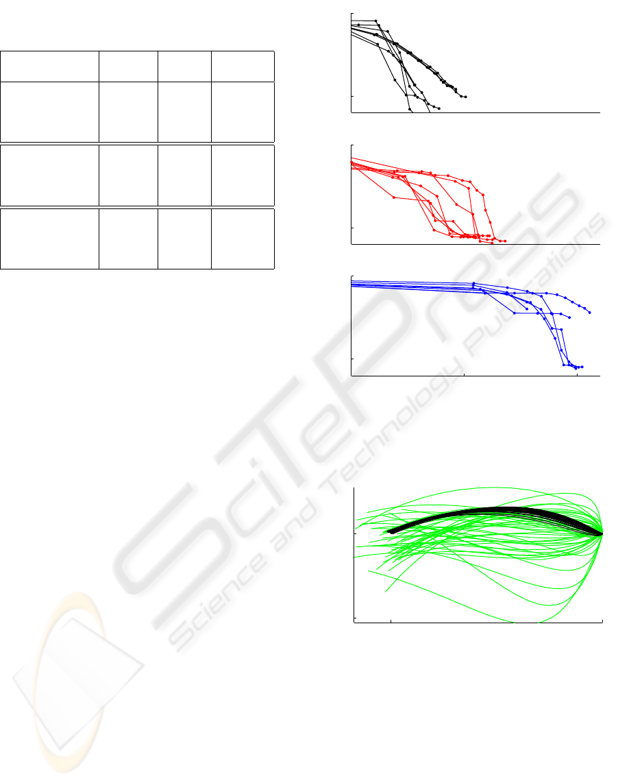
Table 1: Comparison of Four Methods
Method Time Iteration
(sec)
ODE 11.20 N/A
Torque control CGD 8.86 17
arm DDP 2.65 15
ILQR 0.41 6
ODE >400 N/A
Muscle control CGD 91.14 14
arm DDP 181.39 15
ILQR 8.31 8
ODE 6.33 N/A
Inverted CGD 4.95 9
pendulum DDP 1.61 20
ILQR 0.26 5
neighborhood of the nominal trajectory, using second
order approximations. See (Todorov and Li, 2003) for
more detailed descriptions of these preexisting algo-
rithms.
All algorithms were implemented in Matlab, and
used the same dynamic simulation. Table 1 compares
the CPU time and number of iterations for all algo-
rithms on all three problems. Note that the time per
iteration varies substantially (and in the case of ODE
the number of iterations is not even defined) so the
appropriate measure of efficiency is the CPU time.
On all problems studied, the new ILQR method
converged faster than the three existing methods, and
found a better solution. The speed advantage is most
notable in the complex arm model, where ILQR out-
performed the nearest competitor by more than a fac-
tor of 10.
Fig 4 illustrates how the cost of the nominal tra-
jectory decreases with the number of iterations for 8
different initial conditions. Compared with CGD and
DDP method, the new ILQR method converged faster
than the other methods, and found a better solution.
Also we have found that the amount of computation
per iteration for ILQR method is much less than the
other methods. This is because gradient descent re-
quires a linesearch (without which it works poorly);
the implementation of DDP uses a second-order ap-
proximation to the system dynamics and Levenberg-
Marquardt algorithm to compute the inverse matrix
– both of which take a significant amount of time to
compute.
Trajectory-based algorithms related to Pontryagin’s
Maximum Principle in general find locally-optimal
solutions, and complex control problems may exhibit
many local minima. It is useful to address the pres-
ence of local minima. Fig 5 shows how the cloud of
100 randomly initialized trajectories gradually conve-
−5
0
−5
0
1 10 100
−5
0
CPU time (sec)
Log
10
Cost
iLQR
CGD
DDP
Figure 4: Cost vs. Iterations for 2-link 6-muscle Model
1 1.5
1.3
1.5
Shoulder angle (rad)
Elbow angle (rad)
Figure 5: Trajectories of 2-link 6-muscle Model for differ-
ent initial conditions (Black color describes the top 50%
results, light color describes the bottom 50% results)
rge for the muscle-controlled arm model by using
ILQR method. The black curves describe the top
50% results where the shoulder angle and elbow an-
gle arrive to their desired posture respectively, while
the light curves show the bottom 50% results. There
are local minima, but half the time the algorithm con-
verges to the global minimum. Therefore, it can be
used with a small number of restarts.
ICINCO 2004 - INTELLIGENT CONTROL SYSTEMS AND OPTIMIZATION
228

6 CONCLUSIONS AND FUTURE
WORK
Optimal control theory plays a very important role in
the study of biological movement. Further progress
in the field depends on the availability of efficient
methods for solving nonlinear optimal control prob-
lems. This paper developed a new Iterative Lin-
ear Quadratic Regulator (ILQR) algorithm for opti-
mal feedback control of nonlinear dynamical systems.
We illustrated its application to a realistic 2-link, 6-
muscle arm model, as well as simpler control prob-
lems. The simulation results suggest that the new
method is more effective compared to the three most
efficient methods that we are aware of.
While the control problems studied here are deter-
ministic, the variability of biological movements indi-
cates the presence of large disturbances in the motor
system. It is very important to take these disturbances
into account when studying biological control. In par-
ticular, it is known that the motor noise is control-
dependent, with standard deviation proportional to the
mean of the control signal. Such noise has been mod-
elled in the LQG setting before (Todorov and Jordan,
2002). Since the present ILQR algorithm is an exten-
sion to the LQG setting, it should be possible to treat
nonlinear systems with control-dependent noise using
similar methods.
ACKNOWLEDGEMENTS
This work is supported by the National Institutes of
Health Grant 1-R01-NS045915-01.
REFERENCES
Brown, I. E., Cheng, E. J., and Leob, G. (1999). Mea-
sured and modeled properties of mammalian skeletal
muscle. ii. the effects of stimulus frequency on force-
length and force-velocity relationships. J. of Muscle
Research and Cell Motility, 20:627–643.
Bryson, A. E. and Ho, Y.-C. (1969). Applied Optimal Con-
trol. Blaisdell Publishing Company, Massachusetts,
USA.
Harris, C. and Wolpert, D. (1998). Signal-dependent noise
determines motor planning. Nature, 394:780–784.
Jacobson, D. H. and Mayne, D. Q. (1970). Differential Dy-
namic Programming. Elsevier Publishing Company,
New York, USA.
Lahdhiri, T. and Elmaraghy, H. A. (1999). Design of op-
timal feedback linearizing-based controller for an ex-
perimental flexible-joint robot manipulator. Optimal
Control Applications and Methods, 20:165–182.
Lewis, F. L. and Syrmos, V. L. (1995). Optimal Control.
John Wiley and Sons, New York, USA.
Todorov, E. (2003). On the role of primary motor cortex
in arm movement control. In Progress in Motor Con-
trol III, pages 125–166, Latash and Levin(eds), Hu-
man Kinetics.
Todorov, E. and Jordan, M. (2002). Optimal feedback con-
trol as a theory of motor coordination. Nature Neuro-
science, 11(5):1226–1235.
Todorov, E. and Li, W. (2003). Optimal control meth-
ods suitable for biomechanical systems. In Proceed-
ings of the 25th IEEE Conference on Engineering in
Medicine and Biology Society, Cancun, Mexico.
Y, U., M, K., and R, S. (1989). Formation and control of
optimal trajectory in human multijoint arm movement
- minimum torque-change model. Biological Cyber-
netics, 61:89–101.
ITERATIVE LINEAR QUADRATIC REGULATOR DESIGN FOR NONLINEAR BIOLOGICAL MOVEMENT
SYSTEMS
229