
MINING THE RELATIONSHIPS IN THE FORM OF THE
PREDISPOSING FACTORS AND CO-INCIDENT FACTORS
AMONG NUMERICAL DYNAMIC ATTRIBUTES IN TIME
SERIES DATA SET BY USING THE COMBINATION OF SOME
EXISTING TECHNIQUES
Suwimon Kooptiwoot, M. Abdus Salam
School of Information Technologies, The University of Sydney, Sydney, Australia
Key words: Temporal Mining, Time series data set, numerical data, predisposing factor, co-incident factor
Abstract: Temporal mining is a natural extension of data mining with added capabilities of discovering interesting
patterns, inferring relationships of contextual and temporal proximity and may also lead to possible cause-
effect associations. Temporal mining covers a wide range of paradigms for knowledge modeling and
discovery. A common practice is to discover frequent sequences and patterns of a single variable. In this
paper we present a new algorithm which is the combination of many existing ideas consists of the reference
event as proposed in (Bettini, Wang et al. 1998), the event detection technique proposed in (Guralnik and
Srivastava 1999), the large fraction proposed in (Mannila, Toivonen et al. 1997), the causal inference
proposed in (Blum 1982) We use all of these ideas to build up our new algorithm for the discovery of multi-
variable sequences in the form of the predisposing factor and co-incident factor of the reference event of
interest. We define the event as positive direction of data change or negative direction of data change above
a threshold value. From these patterns we infer predisposing and co-incident factors with respect to a
reference variable. For this purpose we study the Open Source Software data collected from SourceForge
website. Out of 240+ attributes we only consider thirteen time dependent attributes such as Page-views,
Download, Bugs0, Bugs1, Support0, Support1, Patches0, Patches1, Tracker0, Tracker1, Tasks0, Tasks1 and
CVS. These attributes indicate the degree and patterns of activities of projects through the course of their
progress. The number of the Download is a good indication of the progress of the projects. So we use the
Download as the reference attribute. We also test our algorithm with four synthetic data sets including noise
up to 50 %. The results show that our algorithm can work well and tolerate the noise data.
1 INTRODUCTION
Time series mining has wide range of applications
and mainly discovers movement pattern of the data,
for example stock market, ECG(Electro-
cardiograms) weather patterns, etc. There are four
main types of movement of data: 1. Long-term or
trend pattern 2. Cyclic movement or cyclic variation
3. Seasonal movement or seasonal variation 4.
Irregular or random movements.
Full sequential pattern is kind of long term or
trend movement, which can be cyclic pattern like
machine working pattern. The idea is to catch the
error pattern which is different from the normal
pattern in the process of that machine. For trend
movement, we try to find the pattern of change that
can be used to estimate the next unknown value at
the next time point or in any specific time point in
the future.
A periodic pattern repeats itself throughout the
time series and this part of data is called a segment.
The main idea is to separate the data into piecewise
periodic segments.
There can be a problem with periodic
behavior within only one segment of time series data
or seasonal pattern. There are several algorithms to
separate segment to find change point, or event.
There are some works (Agrawal and Srikant
1995; Lu, Han et al. 1998) that applied the Apriori-
like algorithm to find the relationship among
attributes, but these work still point to only one
dynamic attribute. Then we find the association
327
Kooptiwoot S. and Abdus Salam M. (2004).
MINING THE RELATIONSHIPS IN THE FORM OF THE PREDISPOSING FACTORS AND CO-INCIDENT FACTORS AMONG NUMERICAL DYNAMIC
ATTRIBUTES IN TIME SERIES DATA SET BY USING THE COMBINATION OF SOME EXISTING TECHNIQUES.
In Proceedings of the Sixth International Conference on Enterprise Information Systems, pages 327-334
DOI: 10.5220/0002625903270334
Copyright
c
SciTePress

among static attributes by using the dynamic
attribute of interest. The work in (Tung, Lu et al.
1999) proposed the idea of finding inter-transaction
association rules such as
RULE1: If the prices of IBM and SUN go up,
Microsoft’s will most likely (80 % of time) go up
the next day.
Event detection from time series data (Guralnik
and Srivastava 1999) utilises the interesting event
detection idea, that is, a dynamic phenomenon is
considered whose behaviour changes over time to be
considered as a qualitatively significant change.
It is interesting if we can find the relationship
among dynamic attributes in time series data which
consist of many dynamic attributes in numerical
form. We attempt to find the relationship that gives
the factors that can be regarded as the cause and
effect of the event of interest. We call these factors
as the predisposing and co-incident factors with
respect to a reference variable. The predisposing
factor can tell us the event of other dynamic
attributes which mostly happen before the reference
event happens. And the co-incident factor can tell us
the event of other dynamic attributes which mostly
happens at the same time or a little bit after the
reference event happens.
2 TEMPORAL MINING
An interesting work in (Roddick and Spiliopoulou
2002), they review research related to the temporal
mining and their contributions related to various
aspects of the temporal data mining and knowledge
discovery and also briefly discuss the relevant
previous work .
In majority of time series analysis, we either
focus on prediction of the curve of a single time
series or the discovery of similarities among
multiple time series. We call time dependent
variable as dynamic variable and call time
independent variable as static variable.
Trend analysis focuses on how to estimate the
value of dynamic attribute of interest at the next time
point or at a specific time point in the future.
There are many kinds of patterns depending on
application data. We can separate pattern types into
four groups.
1. Cyclic pattern is the pattern which has the
exact format and repeat the same format to be cyclic
form, for example, ECG, tidal cycle, sunrise-sunset
2. Periodic pattern is the pattern which has the
exact format in only part of cycle and repeat this
exact format at the same part of cycle, for example,
“Everyday morning at 7:30-8:00 am., Sandy has
breakfast”, the rest of the day Sandy has many
activities which no exact pattern. The cycle of the
day, every day the exact format happen only in the
morning at 7:30-8:00 am.
3. Seasonal pattern is the pattern which is a sub
type of cyclic pattern and periodic pattern. There is a
pattern at a specific range of time during the year’s
cycle, for example, half year sales, fruit season, etc.
4. Irregular pattern is the pattern which doesn’t
have the exact pattern in cycle, for example, network
alarm, computer crash.
2.1 Trend analysis problem
Trend analysis works are normally done by finding
the cyclic patterns of one numerical dynamic
attribute of interest. Once we know the exact pattern
of this attribute, we can forecast the value of this
attribute in the future. If we cannot find the cycle
pattern of this attribute, we can use moving average
window or exponential moving average window
(Weiss and Indurkhya 1998; Kantardzic 2003) to
estimate the value of this dynamic attribute at the
next time point or at the specific time point in the
future.
2.2 Pattern finding problem
In pattern finding problem, we have to find the
change point to be the starting point and the end
point of cycle or segment. Then we try to look for
the segment or cycle pattern that is repeated in the
whole data set. To see which type of pattern it is,
that is, the cyclic pattern of periodic pattern,
seasonal pattern or irregular pattern and observe the
pattern.
The pattern matching problem is to find the way
of matching the segment patterns. Pattern matching,
can be exact pattern (Dasgupta and Forrest 1995) or
rough pattern matching (Hirano, Sun et al. 2001;
Keogh, Chu et al. 2001; Hirano and Tsumoto 2002),
depending on the data application. The exact pattern
is, for example, the cycle of machine working. The
rough pattern is, for example, the hormone level in
human body.
Another problem is the multi-scale pattern
matching problem as seen in (Ueda and S.Suzuki
1990; Hirano, Sun et al. 2001; Hirano and Tsumoto
2001) to match patterns in different time scales.
One interesting work is Knowledge discovery in
Time Series Databases (Last, Klein et al. 2001) .
Last et al. proposed the whole process of knowledge
discovery in time series data bases. They used signal
processing techniques and the information-theoretic
fuzzy approach. The computational theory of
perception (CTP) is used to reduce the set of
extracted rules by fuzzification and aggregation.
ICEIS 2004 - ARTIFICIAL INTELLIGENCE AND DECISION SUPPORT SYSTEMS
328

Another interesting work done in time series
(Keogh, Lonardi et al. 2002) proposed an algorithm
that detects surprising patterns in a time series
database in linear space and time. This algorithm is
named TARZAN. The definition of surprising in this
algorithm is general and domain independent,
describing a pattern as surprising if the frequency
with which we encounter it differs greatly from that
expected given previous experience.
3 PROBLEM
We get an OSS data set from http://sourceforge.net
which is the world’s largest Open Source software
development website. There are 1,097,341 records,
41,540 projects in this data set. This data set consists
of seventeen attributes include time attribute. The
time attribute of each record in this data set is
monthly. Each project in this data set is a software.
There are many attributes that show various
activities. We are interested in thirteen attributes
which indicate the number of activities in this data
set. The data of these thirteen attributes are all
numeric. The value of the Download attribute is the
number of the downloads. So the Download attribute
is the indicator showing how popular the software is
and show how successful the development of the
software is. We are interested in the significant
change of the number of the Download attribute.
Then we employ the idea of the event detection
technique proposed by (Guralnik and Srivastava
1999) to detect the event of the Download attribute.
The event of our interest is the direction of the
significant change of the data which can be up or
down.
We want to find the predisposing factor and the
co-incident factor of the Download event. We
employ the same idea about the reference event as
proposed in (Bettini, Wang et al. 1998) which is the
fixed event of interest and we want to find the other
events related to the reference event. So we call the
Download attribute as the reference attribute and call
the event of the Download attribute as the reference
event.
The predisposing factor of the reference event
can possibly be the cause of the reference event or
the cause of the other event which is the cause of the
reference event. And the co-incident factor of the
reference event can possibly be the effect of the
reference event or the effect of the other event which
is the effect of the reference event somehow or be
the event happening at the same time as the
reference event happens or can be the result from the
same cause of the reference event or just be the
result from the other event which happens at the
same time of the reference event happens. To make
this concept clear, see the example as follow
H I
B
C
ED
F
GK
J
A
L
time
Figure1: The relationships among the events over time
If we have the event A, B, C, D, E, F, G, H, I, J,
K, L and the relationships among them as shown in
Figure 1. That is H and I give B; A and B give C; D
and E give F; C and F give G; J and C give K; K
and G give L. But in our data set consists of only A,
C, F, G, H, L. And the reference event is C. We can
see that H and A happen before C, we may say that
A is the cause of C and/or H is the cause of C. But in
the real relationship as shown above, we know that
H is not the cause of C directly or it is not because A
and H give C. So we call A and H are the
predisposing factors of C. And we find that F
happens at the same time as C happens. And G and
L happen after C. We call F as the co-incident factor
of C. We can see from the relationship that G is the
result from C and F. L is the result from G which is
the result from C. And F is the co-factor of C that
gives G. Only
G is the result from C directly. L is
the result from G which is the result from C.
We want to find the exact relationships among
these events. Unfortunately, no one can guarantee
that our data set of consideration consists of all of
the related factors or events. We can see from the
diagram or the relationship shown in the example
that the relationship among the events can be
complex. And if we don’t have all of the related
events, we cannot find all of the real relationships.
So what we can do with the possible incomplete data
set is mining the predisposing factor and co-incident
factor of the reference event. Then the users can
further consider these factors and collect more data
which related to the reference event and explore
more in depth by themselves on the expert ways in
their specific fields.
The main idea in this part is the predisposing
factor can possibly be the cause of the reference
event and the co-incident factor can possible be the
effect of the reference event. So we employ the same
idea as proposed in (Blum 1982; Blum 1982) that
the cause happens before the effect. The effect
happens after the cause. We call the time point when
the reference event happens as the current time
point. We call the time point before the current time
point as the previous time point. And we call the
MINING THE RELATIONSHIPS IN THE FORM OF THE PREDISPOSING FACTORS AND CO-INCIDENT
FACTORS AMONG NUMERICAL DYNAMIC ATTRIBUTES IN TIME SERIES DATA SET BY USING THE
COMBINATION OF SOME EXISTING TECHNIQUES
329

time point after the current time point as the post
time point. Then we define the predisposing factor
of the reference event as the event which happens at
the previous time point. And we define the co-
incident factor of the reference event as the event
happens at the current time point and/or the post
time point.
4 BASIC DEFINITIONS AND
FRAMEWORK
The method to interpret the result is selecting the
large fraction of the positive slope and the negative
slope at each time point. If it is at the previous time
point that means it is the predisposing factor. If it is
at the current time point and/or the post time point
that means it is the co-incident factor.
Definition1: A time series data set is a set of records
r such that each record contains a set of attributes
and a time attribute. The value of time attribute is
the point of time on time scale such as month, year.
r
j
= { a
1
, a
2
, a
3
, …, a
m
, t
j
}
where
r
j
is the j
th
record in data set
Definition 2: There are two types of the attribute in
time series data set. Attribute that depends on time is
dynamic attribute (
), other wise, it is static attribute
(S).
Definition 3: Time point (t
i
) is the time point on
time scale.
Definition 4: Time interval is the range of time
between two time points [t
1
, t
2
]. We may refer to the
end time point of interval (t
2
).
Definition 5: An attribute function is a function of
time whose elements are extracted from the value of
attribute i in the records, and is denoted as a function
in time, a
i
(t
x
)
a
i
(t
x
) = a
i
r
j
where
a
i
attribute i;
t
x
time stamp associated with this record
Definition 6: A feature is defined on a time interval
[t
1
,t
2
], if some attribute function a
i
(t) can be
approximated to another function Φ (t) in time , for
example,
a
i
(t) Φ (t) , t [t
1
,t
2
]
We say that Φ and its parameters are features of a
i
(t)
in that interval [t
1
,t
2
].
If Φ(t) = α
i
t + β
i
in some intervals, we can say that
in the interval, the function a
i
(t) has a slope of α
i
where slope is a feature extracted from a
i
(t) in that
interval
Definition 7: Slope (α
i
) is the change of value of a
dynamic attribute (a
i
) between two adjacent time
points.
α
i
= ( a
i(
t
x)
- a
i(
t
x-1)
) / t
x
- t
x-1
where
a
i(
t
x)
is the value of a
i
at the time point t
x
a
i
(t
x-1
)is the value of a
i
at the time point t
x-
1
Definition 8: Slope direction d(
i
) is the direction
of slope.
If α
i
> 0, we say d
α
= 1
If α
i
< 0, we say d
α
= -1
If α
i
≅ 0, we say d
α
= 0
Definition 9: A significant slope threshold (
) is the
significant slope level specified by user.
Definition 10: Reference attribute (a
t
) is the
attribute of interest. We want to find the relationship
between the reference attribute and the other
dynamic attributes in the data set.
Definition 11: An event (E1) is detected if α
i
Definition 12: Current time point (t
c
) is the time
point at which reference variable’s event is detected.
Definition 13: Previous time point (t
c-1
) is the
previous adjacent time point of t
c
Definition 14: Post time point (t
c+1
) is the post
adjacent time point of t
c
Proposition 1: Predisposing factor of a
t
denoted as
PE1a
t
is an ordered pair (a
i ,
d
α
) when a
i
If
np
a
i
t
c-1
>
nn
a
i
t
c-1
, then PE1a
t
(a
i
, 1)
If
np
a
i
t
c-1
<
nn
a
i
t
c-1
, then PE1a
t
(a
i
, -1)
where
np
a
i
t
c-1
is the number of positive slope of E1 of a
i
at
t
c-1
nn
a
i
t
c-1
is the number of negative slope of E1of a
i
at
t
c-1
Proposition 2: Co-incident factor of a
t
denoted as
CE1a
t
is an ordered pair (a
i ,
d
α
) when a
i
If ((
np
a
i
t
c
>
nn
a
i
t
c
)
np
a
i
t
c+1
>
nn
a
i
t
c+1
)) ,
then CE1a
t
(a
i
, 1)
If ((
np
a
i
t
c
<
nn
a
i
t
c
)
np
a
i
t
c+1
<
nn
a
i
t
c+1
)) ,
then CE1a
t
(a
i
, -1)
where
np
a
i
t
c
is the number of positive slope of E1 of a
i
at t
c
nn
a
i
t
c
is the number of negative slope of E1 of a
i
at t
c
np
a
i
t
c+1
is the number of positive slope of E1 of a
i
at
t
c+1
nn
a
i
t
c+1
is the number of negative slope of E1 of a
i
at
t
c+1
5 ALGORITHM
Now we present a new algorithm.
Input: The data set which consists of numerical
dynamic attributes. Sort this data set in ascending
order by time, a
t
,
Output:
np
a
i
t
c-1 ,
nn
a
i
t
c-1
,
np
a
i
t
c ,
nn
a
i
t
c
,
np
a
i
t
c+1 ,
nn
a
i
t
c+1
, PE1a
t
, CE1a
t
ICEIS 2004 - ARTIFICIAL INTELLIGENCE AND DECISION SUPPORT SYSTEMS
330
Method:
For all a
i
For all time interval [t
x
, t
x+1
]
Calculate α
i
For a
t
If α
t
Set that time point as t
c
Group record of 3 time points t
c-1
t
c
t
c+1
Count
np
a
i
t
c-1 ,
nn
a
i
t
c-1
,
np
a
i
t
c ,
nn
a
i
t
c
,
np
a
i
t
c+1 ,
nn
a
i
t
c+1
// interpret the result
If
np
a
i
t
c-1
>
nn
a
i
t
c-1
, then PE1a
t
(a
i
, 1)
If
np
a
i
t
c-1
<
nn
a
i
t
c-1
, then PE1a
t
(a
i
, -1)
If
np
a
i
t
c
>
nn
a
i
t
c
, then CE1a
t
(a
i
, 1)
If
np
a
i
t
c
<
nn
a
i
t
c
, then CE1a
t
(a
i
, -1)
If
np
a
i
t
c+1
>
nn
a
i
t
c+1
, then CE1a
t
(a
i
, 1)
If
np
a
i
t
c+1
<
nn
a
i
t
c+1
, then CE1a
t
(a
i
, -1)
For the event, the data change direction, we
employ the method proposed by (Mannila, Toivonen
et al. 1997) that is using the large fraction to judge
the data change direction of the attribute of
consideration.
Using the combination of the ideas mentioned
above, we can find the predisposing factor and the
co-incident factor of the reference event of interest.
The steps to do this task are
1. Set the threshold of the data change of the
reference attribute.
2. Use this data change threshold to find the event
which is the change of the data of the reference
attribute between two adjacent time point is
equal to or higher than the threshold, and mark
that time point as the current time point
3. Look at the previous adjacent time point to find
the predisposing factor and the post adjacent
time point of the current time point to find the
co-incident factor
4. Separate the case of the reference event to be
the positive direction and the negative direction
4.1 For each case, count the number of the positive
change direction and the number of the negative
change direction of the other attributes in
consideration.
4.2 Select the large fraction between the number of
the positive change direction and the number of
the negative change direction. If the number of
the positive direction is larger than the number
of the negative direction, we say that the
positive change direction of the considered
attribute is the factor. Otherwise, we say that the
negative change direction of the considered
attribute is the factor. If the factor is found at the
previous time point, we say that the factor is the
predisposing factor. If the factor is found at the
current time point or the post time point, we say
that the factor is the co-incident factor.
We don’t use the threshold to find the event of
the other attributes because of the idea of the degree
of importance (Salam 2001). For example, the
effects of the different kind of chilly on our food are
different. Only small amount of the very hot chilly
make our food very hot. Very much of sweet chilly
make our food not so spicy. We see that the same
amount of the different kind of chilly creates the
different level of the hotness in our food. The very
hot chilly has the degree of importance in our food
higher than the sweet chilly. Another example, about
the number of Download of the software A, we can
see that normal factors effect on the number of
Download are still there. But in case there is a
lecturer or a teacher assign his/her 300 students in
his/her class to test the software A and report the
result to him/her within 2 weeks. This assignment
makes the number of Download of the software A
increase significantly in very short time. For the
other software, software B, is in the same situation
or the same quality or the same other factors as the
software A which should get the same number of
Download as the software A, but there is no lecturer
or teacher assigning his/her 300 students to test it.
The number of Download of the software B is lower
than the software A. Or in case there is a teacher or
lecturer assign his/her 500 students to test 2 or 3
softwares and report the results to him/her within
one month. This event makes the number of
Download of many softwares increase in very short
time. Such incidental factors have the potential to
skew the results. Such factors may have high degree
of importance that effect on the number of
Download of the software. It is the same as the only
small amount of the data change of some attributes
can make the data of the reference attribute change
very much. So we do not specify the threshold of the
event of the other attributes to be considered as the
predisposing factor or the co-incident factor. For
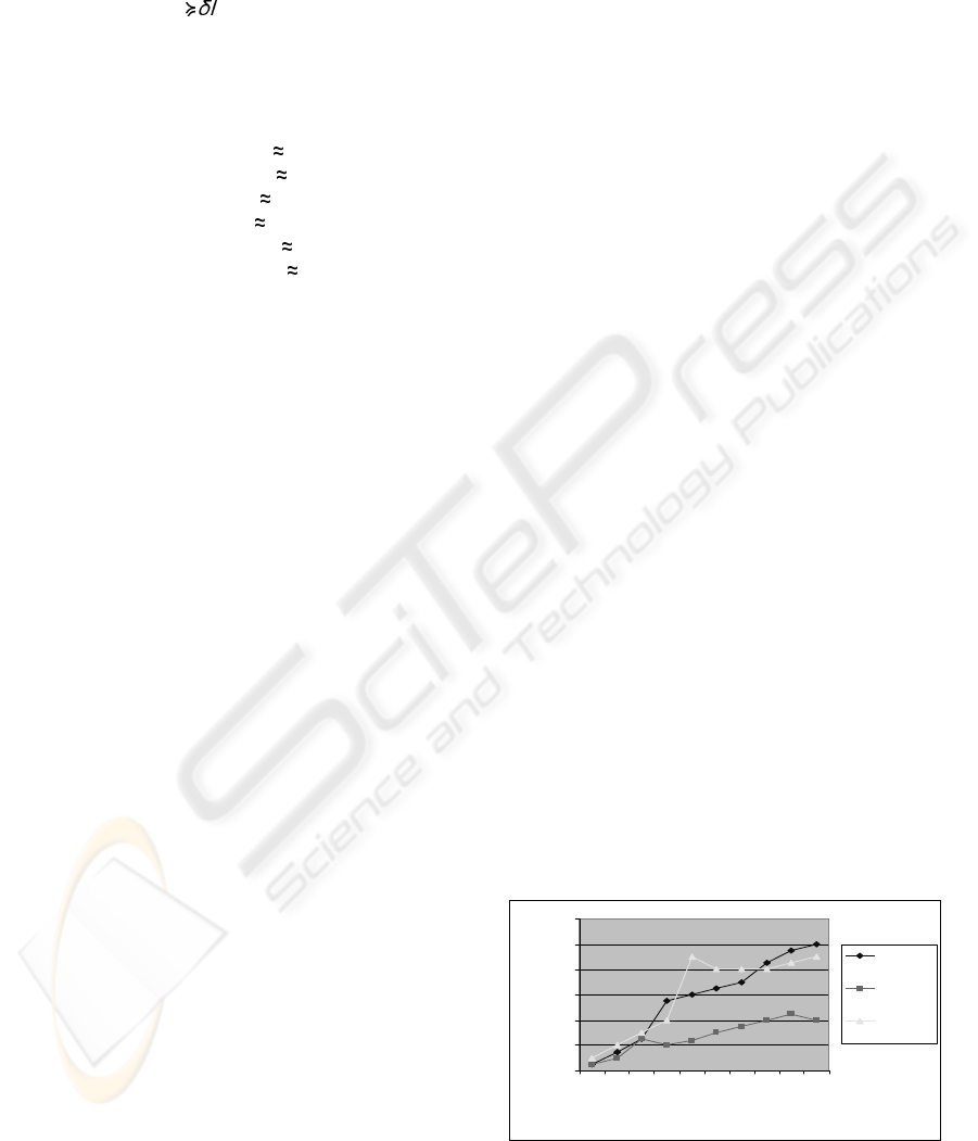
example, the graph of the data is shown in Graph 1
0
20
40
60
80
100
120
1/3/2003
2/3/2003
3/3/2003
4/3/2003
5/3/2003
6/3/2003
7/3/2003
8/3/2003
9/3/2003
10/3/2003
reference
attribute
a2
a3
Graph 1: the data in the graph
MINING THE RELATIONSHIPS IN THE FORM OF THE PREDISPOSING FACTORS AND CO-INCIDENT
FACTORS AMONG NUMERICAL DYNAMIC ATTRIBUTES IN TIME SERIES DATA SET BY USING THE
COMBINATION OF SOME EXISTING TECHNIQUES
331

We calculate the slope value showing how much
the data change and the direction of the data change
per time unit.
Then we set the data change threshold as 15. We
use this threshold to find the reference event. We
find the reference event at the time 4/03. Then we
mark this time point as the current time point. Next
we look at the previous time point, 3/03, for the
predisposing factor, we find that a2 with the positive
direction and a3 with positive direction are the
predisposing factor of the reference event. Then we
look at the current time point and the post time
point, 4/03 and 5/03, for the co-incident factor, we
find that at the current time point, a2 with the
negative direction and a3 with the positive direction
are the co-incident factor. And at the post time point,
a2 with the positive direction and a3 with the
positive direction are the co-incident factor. We can
summarize the result in the pattern table as shown in
Table 1.
Table 1: the direction of each attribute at each time point
Previous
time point
Current
time point
Post time
point
a2 Up down up
a3 Up up up
6 OSS DATA
The OSS data on SourceForge website has been
collected over the last few years. Initially some
projects were listed with the SourceForge at various
developmental stages. Since then a large number of
new projects have been added at different time
points and are progressing at different pace. Though
they are at different developmental stages, there data
is still collected at regular intervals of one month.
Due to this a global comparison of all of the projects
poses many problems. Here we wish to explore
local trends at each event.
The main idea is to choose an event in the
reference variable as a reference time point and mine
the relationship with other numerical dynamic
attributes. By using this method, we wish to explore
the predisposing and co-incident factors of the
reference event of interest in time series data set.
The predisposing factor is the factor which can be
the cause of the reference event or the factor that has
effect on the reference event somehow. The co-
incident factor is the factor that can be the effect of
the reference attribute or the factor that is also the
result of the predisposing factor of the reference
event or the reference event effect on it somehow.
7 EXPERIMENTS
We apply our method with one OSS data set which
consists of 17 attributes (Project name, Month-Year,
Rank0, Rank1, Page-views, Download, Bugs0,
Bugs1, Support0, Support1, Patches0, Patches1,
Tracker0, Tracker1, Tasks0, Tasks1, CVS. This data
set consists of 41,540 projects, 1,097,341 records
7.1 Results
We select the Download attribute to be the reference
attribute. And we set the significant data change
threshold as 50. The results are separated into two
cases. The first case is the data change direction of
the Download is positive. The second is the data
change direction of the Download is negative. The
results are shown in Table 2 and Table 3
accordingly.
7.1.1 Slope direction of the Download is
positive
Table 2: Summary of the results in case the slope direction
of the Download is positive
previous current post
P/V Up up down
Bugs0 Up up down
Bugs1 Up up down
Support0 up up down
Support1 up up down
Patches0 up up down
Patches1 up up down
Tracker0 up up down
Tracker1 up up down
Tasks0 down down down
Tasks1 up up down
CVS up up down
From this finding we can see that the predisposing
factors of the number of the Download significantly
increases are the number of Tasks0 decreases and
the rest of other attributes which consists of Page
views, Bugs0, Bugs1, Support0, Support1, Pathces0,
Patches1, Tracker0, Tracker1, Tasks1, CVS
increase. At the same time interval, the co-incident
ICEIS 2004 - ARTIFICIAL INTELLIGENCE AND DECISION SUPPORT SYSTEMS
332

factors of the number of Download significantly
increases are the same as its predisposing factors but
after that the number of all of the other attributes
decreases.
7.1.2 Slope direction of the Download is
negative
Table 3: Summary of the result in case the slope direction
of the Download is negative
previous current post
P/V up down down
Bugs0 up down down
Bugs1 up down up
Support0 up down down
Support1 up down up
Patches0 up down up
Patches1 up down up
Tracker0 up down down
Tracker1 up down up
Tasks0 down down down
Tasks1 down down down
CVS down down down
From these results, we find that the predisposing
factors of the number of the Download significantly
decreases are the number of almost all of the other
attributes increases, except only the number of
Tasks0, Tasks1 and CVS decrease. And the co-
incident factors of the number of Download
significantly decrease are the number of all of the
other attributes decrease at the same time interval.
After that the number P/V, Bugs0, Support0,
Tracker0, Tasks0, Tasks1, CVS decrease and the
number of Bugs1, Support1, Patches0, Patches1,
Tracker1 increase .
8 PERFORMANCE
Our methods consume time to find the predisposing
factor and the co-incident factor of the reference
event just in O(n) where n is the number of the total
records. The most time consuming is the time for
calculating the slope (the data change) of every two
adjacent time points of the same project which take
time O(n). And we have to spend time to select the
reference event by using the threshold which takes
time O(n). We have to spend time to group records
around the reference event (at the previous time
point, the current time point and the post time point)
which is O(n). And the time for counting the number
of events of the other attributes at each time point
around the current time point is O(n). The time in
overall process can be approximate to O(n), which is
not exponential. So our methods are good enough to
apply in the big real life data set.
In our experiments we use PC PentiumIV 1.6
GHz, RAM 1 GB. The operating system is MS
WindowsXP Professional. We implement these
algorithms in Perl 5.8 on command line. The data set
test has 1,097,341 records, 41, 540 projects with
total 17 attributes. The number of attributes of
consideration is 13 attributes. The size of this data
set is about 48 MB.
We want to see if our program consume running
time in linear scale with the size of the data or not.
Then we test with the different number of records in
each file and run each file at a time. The result is
shown in Graph 2.
time(sec)
0
5
10
15
20
25
30
35
40
45
50
6000 8000 10000 12000 14000 16000
time(sec)
Graph 2: Running time (in seconds) and the number of
records to be run at a time
From this result confirm us that our algorithm
consumes execution time in linear scale with the
number of records.
8.1 Accuracy test with Synthetic Data
sets
We synthesize 4 data sets as follow
1. Correct complete data set
2. Put 5 % of noise in the first data set
3. Put 20 % of noise in the first data set
4. Put 50 % of noise in the first data set
We set the data change threshold as 10. The
result is almost all of four data sets correct, except
only at the third data set with 20 % of noise, there is
only one point in the result different from the others,
that is, the catalyst at the current point changes to be
positive slope instead of steady.
MINING THE RELATIONSHIPS IN THE FORM OF THE PREDISPOSING FACTORS AND CO-INCIDENT
FACTORS AMONG NUMERICAL DYNAMIC ATTRIBUTES IN TIME SERIES DATA SET BY USING THE
COMBINATION OF SOME EXISTING TECHNIQUES
333

9 CONCLUSION
The combination of the existing methods to be our
new algorithm can be used to mine the predisposing
factor and co-incident factor of the reference event
very well. As seen in our experiments, our proposed
algorithm can be applied to both the synthetic and
the real life data set. The performance of our
algorithm is also good. They consume execution
time just in linear time scale and also tolerate to the
noise data.
10 DISCUSSION
The threshold is the indicator to select the event
which is the significant change of the data of the
attribute of consideration. When we use the different
thresholds in detecting the events, the results can be
different. So setting the threshold of the data change
have to be well justified. It can be justified by
looking at the data and observing the characteristic
of the attributes of interest. The users have to realize
that the results they get can be different depending
on their threshold setting. The threshold reflects the
degree of importance of the predisposing factor and
the co-incident factor to the reference event. If the
degree of importance of an attribute is very high,
just little change of the data of that attribute can
make the data of the reference attribute change very
much. So for this reason setting the threshold value
is of utmost importance for the accuracy and
reliability of the results.
REFERENCES
Agrawal, R. and Srikant R., 1995. Mining Sequential
Patterns. In Proceedings of the IEEE International
Conference on Data Engineering, Taipei, Taiwan.
Bettini, C., Wang S., et al. 1998. Discovering Frequent
Event Patterns with Multiple Granularities in Time
Sequences. In IEEE Transactions on Knowledge and
Data Engineering 10(2).
Blum, R. L., 1982. Discovery, Confirmation and
Interpretation of Causal Relationships from a Large
Time-Oriented Clinical Databases: The Rx Project.
Computers and Biomedical Research 15(2): 164-187.
Dasgupta, D. and Forrest S., 1995. Novelty Detection in
Time Series Data using Ideas from Immunology. In
Proceedings of the 5th International Conference on
Intelligent Systems, Reno, Nevada.
Guralnik, V. and Srivastava J., 1999. Event Detection from
Time Series Data. In KDD-99, San Diego, CA USA.
Hirano, S., Sun X., et al., 2001. Analysis of Time-series
Medical Databases Using Multiscale Structure
Matching and Rough Sets-Based Clustering
Technique. In IEEE International Fuzzy Systems
Conference.
Hirano, S. and Tsumoto S., 2001. A Knowledge-Oriented
Clustering Technique Based on Rough Sets. In 25th
Annual International Computer Software and
Applications Conference (COMPSAC'01), Chicago,
Illinois.
Hirano, S. and Tsumoto S., 2002. Mining Similar
Temporal Patterns in Long Time-Series Data and Its
Application to Medicine. In IEEE: 219-226.
Kantardzic, M., 2003. Data Mining Concepts, Models,
Methods, and Algorithms. USA, IEEE Press.
Keogh, E., Chu S., et al., 2001. An Online Algorithm for
Segmenting Time Series. In Proceedings of IEEE
International Conference on Data Mining, 2001.
Keogh, E., Lonardi S., et al., 2002. Finding Surprising
Patterns in a Time Series Database in Linear Time
and Space. In Proceedings of The Eighth ACM
SIGKDD International Conference on Knowledge
Discovery and Data Mining (KDD '02), Edmonton,
Alberta, Canada.
Last, M., Klein Y., et al., 2001. Knowledge Discovery in
Time Series Databases. In IEEE Transactions on
Systems, Man, and Cybernetics 31(1): 160-169.
Lu, H., Han J., et al., 1998. Stock Movement Prediction
and N-Dimensional Inter-Transaction Association
Rules. In Proc. of 1998 SIGMOD'98 Workshop on
Research Issues on Data Mining and Knowledge
Discovery (DMKD'98) ,, Seattle, Washington.
Mannila, H., Toivonen H., et al., 1997. Discovery of
frequent episodes in event sequences. In Data Mining
and Knowledge Discovery 1(3): 258-289.
Roddick, J. F. and Spiliopoulou M., 2002. A Survey of
Temporal Knowledge Discovery Paradigms and
Methods. In IEEE Transactions on Knowledge and
Data Mining 14(4): 750-767.
Salam, M. A., 2001. Quasi Fuzzy Paths in Semantic
Networks. In Proceedings 10th IEEE International
Conference on Fuzzy Systems, Melbourne, Australia.
Tung, A., Lu H., et al., 1999. Breaking the Barrier of
Transactions: Mining Inter-Transaction Association
Rules. In Proceedings of the Fifth International on
Knowledge Discovery and Data Mining [KDD 99],
San Diego, CA.
Ueda, N. and Suzuki S., 1990. A Matching Algorithm of
Deformed Planar Curves Using Multiscale
Convex/Concave Structures. In JEICE Transactions on
Information and Systems J73-D-II(7): 992-1000.
Weiss, S. M. and Indurkhya N., 1998. Predictive Data
Mining. San Francisco, California, Morgn Kaufmann
Publsihers, Inc.
ICEIS 2004 - ARTIFICIAL INTELLIGENCE AND DECISION SUPPORT SYSTEMS
334
