
ON THE BALANCING CONTROL OF HUMANOID ROBOT
Youngjin Choi
School of electrical engineering and computer science, Hanyang University, Ansan, 426-791, Republic of Korea
Doik Kim
Intelligent Robotics Research Center, Korea Institute of Science and Technology (KIST), Seoul, 136-791, Republic of Korea
Keywords:
WBC (whole body coordination), Humanoid robot, Posture control, CoM (center of mass) Jacobian.
Abstract:
This paper proposes the kinematic resolution method of CoM(center of mass) Jacobian with embedded mo-
tions and the design method of posture/walking controller for humanoid robots. The kinematic resolution of
CoM Jacobian with embedded motions makes a humanoid robot balanced automatically during movement of
all other limbs. Actually, it offers an ability of WBC(whole body coordination) to humanoid robot. Also, we
prove that the proposed posture/walking controller brings the ISS(disturbance input-to-state stability) for the
simplified bipedal walking robot model.
1 INTRODUCTION
Recently, there have been many researches about hu-
manoid motion control, for example, walking con-
trol(Choi et al., 2006; Kajita et al., 2001), and whole
body coordination(Sugihara and Nakamura, 2002).
Especially, the WBC(whole body coordination) al-
gorithm with good performance becomes the essen-
tial part in the development of humanoid robot be-
cause it offers the enhanced stability and flexibility
to the humanoid motion planning. In this paper, we
suggest the kinematic resolution method of CoM Ja-
cobian with embedded motions, actually, which of-
fers the ability of WBC to humanoid robot. For
example, if humanoid robot stretches two arms for-
ward, then the position of CoM(center of mass) of
humanoid robot moves forward and its ZMP(zero mo-
ment point) swings back and forth. In this case, the
proposed kinematic resolution method of CoM Jaco-
bian with embedded (stretching arms) motion offers
the joint configurations of supporting limb(s) calcu-
lated automatically to maintain the position of CoM
fixed at one point.
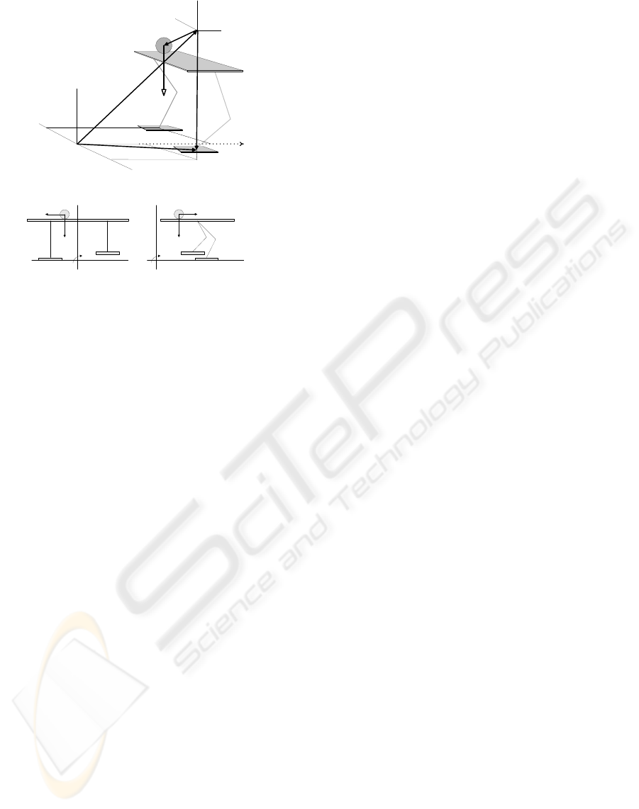
Also, we will simplify the dynamics of bipedal
robot as the equation of motion of a point mass con-
centrated on the position of CoM. First, let us assume
that the motion of CoM is constrained on the surface
z = c
z
, then the rolling sphere model with the concen-
trated point mass m can be obtained as the simplified
model for bipedal robot as shown in Fig. 1. The mo-
tion of the rolling sphere on a massless plate is de-
scribed by the position of CoM, c = [c
x
,c
y
,c
z
]
T
, and
the ZMP is described by the position on the ground,
p = [p
x
, p
y
,0]
T
. Second, let us take the moments
about origin on the ground of the linear equations of
motion for the rolling sphere (with a point mass = m)
confined to motion on a plane z = c
z
as shown in Fig.
1, then the following equations are obtained:
τ
x
= mgc
y
−m¨c
y
c
z
(1)
τ
y
= −mgc
x
+ m¨c
x
c
z
(2)
τ
z
= −m¨c
x
c
y
+ m¨c
y
c
x
(3)
where g is the acceleration of gravity, c
z
is a height
constant of constraint plane and τ
i
is the moment
about i-coordinate axis, for i = x,y,z. Now, if we in-
troduce the conventional definition of ZMP as follow-
ing forms:
p
x
△
= −
τ
y
mg
and p
y
△
=
τ
x
mg
to two equations (1) and (2), then ZMP equations can
be obtained as two differential equations:
p
i
= c
i
−
1
ω
2
n
¨c
i
for i = x,y (4)
where ω
n
△
=
p
g/c
z
is the natural radian frequency of
the simplified biped walking robot system. Above
248
Choi Y. and Kim D. (2007).
ON THE BALANCING CONTROL OF HUMANOID ROBOT.
In Proceedings of the Fourth International Conference on Informatics in Control, Automation and Robotics, pages 248-252
DOI: 10.5220/0001623302480252
Copyright
c
SciTePress
CoM(c
x
,c
y
,c
z
)
Supporting
Foot
Y
X
Z
O
Walking
Direction
Shifting
Foot
World Coordinate
Frame
Body Center
Frame
Z
Y
Z
X
y
mc
ɺɺ
g
m
−
g
m
−
x
τ
CoM(c
y
,c
z
)
x
mc
ɺɺ
g
m
−
CoM(c
x
,c
z
)
y
τ
x
ZMP(p
y
)
x
ZMP(p
x
)
o
r
o
o
i
R r
i
r
Figure 1: Rolling Sphere Model for Dynamic Walking.
equations will be used to prove the stability of the
posture/walking controller in the following sections.
2 KINEMATIC RESOLUTION
Let a robot has n limbs and the first limb be the base
limb. The base limb can be any limb but it should be
on the ground to support the body. Each limb of a
robot is hereafter considered as an independent limb.
In general, the i-th limb has the following relation:
o
˙x
i
=
o
J
i
˙q
i
(5)
for i = 1,2,··· ,n, where
o
˙x
i
∈ ℜ
6
is the velocity of
the end point of i-th limb, ˙q
i
∈ ℜ
n
i
is the joint ve-
locity of i-th limb,
o
J
i
∈ ℜ
6×n
i
is the usual Jacobian
matrix of i-th limb, and n
i
means the number of active
links of i-th limb. The leading superscript o implies
that the elements are represented on the body center
coordinate system shown in Fig. 1, which is fixed on
a humanoid robot.
In the humanoid robot, the body center is floating,
and thus the end point motion of i-th limb about the
world coordinate system is written as follows:
˙x
i
= X
−1
i
˙x
o
+ X
o
o
J
i
˙q
i
(6)
where ˙x
o
= [˙r
T
o
;ω
o
T
]
T
∈ℜ
6
is the velocity of the body
center represented on the world coordinate system,
and
X
i
=
I
3
[R
o
o
r
i
×]
0
3
I
3
∈ ℜ
6×6
(7)
is a (6 ×6) matrix which relates the body center ve-
locity and the i-th limb velocity. I
3
and 0
3
are an
(3 ×3) identity and zero matrix, respectively. R
o
o
r
i
is the position vector from the body center to the end
point of the i-th limb represented on the world coordi-
nate frame. [(·)×] is a skew-symmetric matrix for the
cross product. The transformation matrix X
o
is
X
o
=
R
o
0
3
0
3
R
o
∈ ℜ
6×6
(8)
where R
o
∈ℜ
3×3
is the orientation of the body center
represented on the world coordinate frame, and here-
after, we will use the relation J
i
△
= X
o
o
J
i
.
All the limbs in a robot should have the same body
center velocity, in other words, from Eq. (6), we can
see that all the limbs should satisfy the compatibility
condition that the body center velocity is the same,
and thus, i-th limb and j-th limb should satisfy the
following relation:
X
i
(˙x
i
−J
i
˙q
i
) = X
j
(˙x
j
−J
j
˙q
j
). (9)
From Eq. (9), the joint velocity of any limb can be
represented by the joint velocity of the base limb and
cartesian motions of limbs. Actually, the base limb
should be chosen to be the support leg in single sup-
port phase or one of both legs in double support phase.
Let us express the base limb with the subscript 1, then
the joint velocity of i-th limb is expressed as:
˙q
i
= J
+
i
˙x
i
−J
+
i
X
i1
(˙x
1
−J
1
˙q
1
), (10)
for i = 2,··· ,n, where J
+
i
means the Moore-Penrose
pseudoinverse of J
i
and
X
i1
△
= X
−1
i
X
1
=
I
3
[R
o
(
o
r
1
−
o
r
i
)×]
0
3
I
3
. (11)
The position of CoM represented on the world co-
ordinate frame, in Fig. 1, is given by
c = r
o
+
n
∑
i=1
R
o
o
c
i
(12)
where n is the number of limbs, c is the position vec-
tor of CoM represented on the world coordinate sys-
tem, and
o
c
i
means the CoM position vector of i-th
limb represented on the body center coordinate frame
which is composed of n
i
active links. Now, let us dif-
ferentiate Eq. (12), then the it is obtained as follows:
˙c = ˙r
o
+ ω
o
×(c−r
o
) +
n
∑
i=1
R
o
o
J
c
i
˙q
i
. (13)
where
o
J
c
i
∈ ℜ
3×n
i
means CoM Jacobian matrix of
i-th limb represented on the body center coordinate
frame, and hereafter, we will use the relation J
c
i
△
=
R
o
o
J
c
i
.
ON THE BALANCING CONTROL OF HUMANOID ROBOT
249

Remark 1 The CoM Jacobian matrix of i-th limb rep-
resented on the body center frame is expressed by
o
J
c
i
△
=
n
i
∑
k=1
µ
i,k
∂
o
c
i,k
∂q
i
, (14)
where
o
c
i,k
∈ ℜ
3
means the position vector of center
of mass of k-th link in i-th limb represented on the
body center frame and the mass influence coefficient
of k-th link in i-th limb is defined as follow:
µ
i,k
△
=
mass of k-th link in i-th limb
total mass
. (15)
The motion of body center frame can be obtained
by using Eq. (6) for the base limb as follows:
˙x
o
= X
1
{
˙x
1
−J
1
˙q
1
}
˙r
o
ω
o
=
I
3
[R
o
o
r
1
×]
0
3
I
3
˙r
1
ω
1
−
J
v
1
J
ω
1
˙q
1
,
(16)
where J
v
1
and J
ω
1
are the linear and angular velocity
part of the base limb Jacobian J
1
expressed on the
world coordinate frame, respectively. Now, if Eq. (10)
is applied to Eq. (13) for all limbs except the base
limb with subscript 1, the CoM motion is rearranged
as follows:
˙c = ˙r
o
+ ω
o
×(c−r
o
) + J
c
1
˙q
1
+
n
∑
i=2
J
c
i
J
+
i
(˙x
i
−X
i1
˙x
1
) +
n
∑
i=2
J
c
i
J
+
i
X
i1
J
1
˙q
1
. (17)
Here, if Eq. (16) is applied to Eq. (17), then the
CoM motion is only related with the motion of base
limb. Also, if the base limb has the face contact with
the ground (the end-point of base limb represented
on world coordinate frame is fixed, ˙x
1
= 0, namely,
˙r
1
= 0, ω
1
= 0), then Eq. (17) is simplified as follows:
˙c−
n
∑
i=2
J
c
i
J
+
i
˙x
i
= −J
v
1
˙q
1
+ r
c1
×J
ω
1
˙q
1
+ J
c
1
˙q
1
+
n
∑
i=2
J
c
i
J
+
i
X
i1
J
1
˙q
1
. (18)
where r
c1
= c−r
1
.
Finally, 3×n
1
CoM Jacobian matrix with embed-
ded motions can be rewritten like usual kinematic Ja-
cobian of base limb:
˙c
fsem
= J
fsem
˙q
1
, (19)
where
˙c
fsem
△
= ˙c−
n
∑
i=2
J
c
i
J
+
i
˙x
i
, (20)
J
fsem
△
= −J
v
1
+ r
c1
×J
ω
1
+ J
c
1
+
n
∑
i=2
J
c
i
J
+
i
X
i1
J
1
.
(21)
Here, if the CoM Jacobian is augmented with the
orientation Jacobian of body center (ω
o
= −J
ω
1
q
1
)
and all desired cartesian motions are embedded in Eq.
(20), then the desired joint configurations of base limb
(support limb) are resolved as follows:
˙q
1,d
=
J
fsem
−J
ω
1
+
˙c
fsem,d
ω
o,d
, (22)
where the subscript d means the desired motion and
˙c
fsem,d
= ˙c
d
−
∑
n
i=2
J
c
i
J
+
i
˙x
i,d
. (23)
All the given desired limb motions, ˙x
i,d
are embedded
in the relation of CoM Jacobian, thus the effect of the
CoM movement generated by the given limb motion
is compensated by the base limb. The CoM motion
with fully specified embedded motions,
After solving Eq. (22), the desired joint motion of
the base limb is obtained. The resulting base limb mo-
tion makes a humanoid robot balanced automatically
during the movement of the all other limbs. With the
desired joint motion of base limb, the desired joint
motions of all other limbs can be obtained by Eq. (10)
as follow:
˙q
i,d
= J
+
i
(˙x
i,d
+ X
i1
J
1
˙q
1,d
), for i = 2,··· , n. (24)
The resulting motion follows the given desired mo-
tions, regardless of balancing motion by base limb.
In other words, the suggested kinematic resolution
method of CoM Jacobian with embedded motion of-
fers the WBC(whole body coordination) function to
the humanoid robot automatically.
3 STABILITY
The control system is said to be disturbance input-
to-state stable (ISS), if there exists a smooth positive
definite radially unbounded function V(e,t), a class
K
∞
function γ
1
and a class K function γ
2
such that
the following dissipativity inequality is satisfied:
˙
V ≤ −γ
1
(|e|) + γ
2
(|ε|), (25)
where
˙
V represents the total derivative for Lyapunov
function, e the error state vector and ε disturbance in-
put vector.
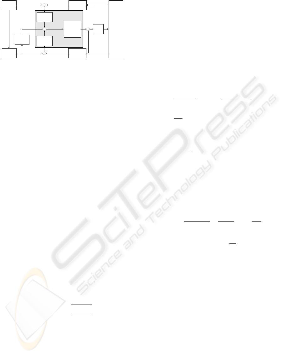
In this section, we propose the posture/walking
controller for bipedal robot systems as shown in Fig.
2. In this figure, first, the ZMP Planer and CoM Planer
generate the desired trajectories satisfying the follow-
ing differential equation:
p
i,d
= c
i,d
−1/ω
2
n
¨c
i,d
for i = x, y. (26)
Second, the simplified model for the real bipedal
walking robot has the following dynamics:
˙c
i
= u
i
+ ε
i
p
i
= c
i
−1/ω
2
n
¨c
i
for i = x, y,
(27)
ICINCO 2007 - International Conference on Informatics in Control, Automation and Robotics
250
CoM
Planner
Des. ZMP
_
ZMP
Planner
CoM
Controller
Actual CoM
+
Des. CoM
Real
Bipedal
Robot
Actual ZMP
p
i
d
c
i
d
c
i
p
i
u
i
ZMP
Controller
_
_
Posture/Walking
Controller
+
Control
Input
c
i
d
.
d/dt
Kinematic
Resolution
of CoM
Jacobian
q
d
Joint
Servo
q
Actual
Configuration
CoM
Calculation
ZMP
Calculation
_
q
F/T
Measured
Force/Torque
Figure 2: Posture/Walking Controller for Humanoid Robot.
where ε
i
is the disturbance input produced by ac-
tual control error, u
i
is the control input, c
i
and p
i
are the actual positions of CoM and ZMP measured
from the real bipedal robot, respectively. Here, we as-
sume that the the disturbance produced by control er-
ror is bounded and its differentiation is also bounded,
namely, |ε
i
| < a and |
˙
ε
i
| < b with any positive con-
stants a and b. Also, we should notice that the control
error always exists in real robot systems and its mag-
nitude depends on the performance of embedded local
joint servos. The following theorem proves the stabil-
ity of the posture/walking controller to be suggested
for the simplified robot model.
Theorem 1 Let us define the ZMP and CoM error for
the simplified bipedal robot control system (27) as fol-
lows:
e
p,i
△
= p
i,d
− p
i
(28)
e
c,i
△
= c
i,d
−c
i
for i = x, y. (29)
If the posture/walking control input u
i
in Fig. 2 has
the following form:
u
i
= ˙c
d
i
−k
p,i
e
p,i
+ k
c,i
e
c,i
(30)
under the gain conditions:
k
c,i
> ω
n
and 0 < k
p,i
<
ω
2
n
−β
2
ω
n
−γ
2
(31)
satisfying the following conditions:
β < ω
n
and γ <
s
ω
2
n
−β
2
ω
n
, (32)
then the posture/walking controller gives the distur-
bance input(ε
i
,
˙
ε
i
)-to-state(e
p,i
,e
c,i
) stability (ISS) to
a simplified bipedal robot, where, the k
p,i
is the pro-
portional gain of ZMP controller and k
c,i
is that of
CoM controller in Fig. 2.
Proof. First, we get the error dynamics from Eq.
(26) and (27) as follows:
¨e
c,i
= ω
2
n
(e
c,i
−e
p,i
). (33)
Second, another error dynamics is obtained by using
Eq. (27) and (30) as follows:
k
p,i
e
p,i
= ˙e
c,i
+ k
c,i
e
c,i
+ ε
i
, (34)
also, this equation can be rearranged for ˙e
c
:
˙e
c,i
= k
p,i
e
p,i
−k
c,i
e
c,i
−ε
i
. (35)
Third, by differentiating the equation (34) and by us-
ing equations (33) and (35), we get the following:
˙e
p,i
= 1/k
p,i
( ¨e
c,i
+ k
c,i
˙e
c,i
+
˙
ε
i
)
= ω
2
n
/k
p,i
(e
c,i
−e
p,i
)
+k
c,i
/k
p,i
(k
p,i
e
p,i
−k
c,i
e
c,i
−ε
i
) + (1/k
p,i
)
˙
ε
i
=
ω
2
n
−k
2
c,i
k
p,i
!
e
c,i
−
ω
2
n
−k
p,i
k
c,i
k
p,i
e
p,i
+
1
k
p,i
(
˙
ε
i
−k
c,i
ε
i
). (36)
Fourth, let us consider the following Lyapunov func-
tion:
V(e
c,i
,e
p,i
)
△
=
1
2
(k
2
c,i
−ω
2
n
)e
2
c,i
+ k
2
p,i
e
2
p,i
, (37)
where V(e
c
,e
p
) is the positive definite function for
k
p,i
> 0 and k
c,i
> ω
n
, except e
c,i
= 0 and e
p,i
= 0.
Now, let us differentiate the above Lyapunov func-
tion, then we can get the following:
˙
V ≤ −(k
c,i
−α
2
)(k
2
c,i
−ω
2
n
)e
2
c,i
−k
p,i
[ω
2
n
−(k
p,i
+ γ
2
)k
c,i
−β
2
]e
2
p,i
+
"
(k
2
c,i
−ω
2
n
)
4α
2
+
k
p,i
k
c,i
4γ
2
#
ε
2
i
+
k
p,i
4β
2
˙
ε
2
i
(38)
where e
2
c,i
term is negative definite with any pos-
itive constant satisfying α <
√
ω
n
and e
2
p,i
term
is negative definite under the given conditions
(31). Here, since the inequality (38) follows the
ISS property (25), we concludes that the pro-
posed posture/walking controller gives the distur-
bance input(ε
i
,
˙
ε
i
)-to-state(e
p,i
,e
c,i
) stability (ISS) to
the simplified control system model of bipedal robot.
To make active use of the suggested control
scheme, the control input u of Eq. (30) suggested in
Theorem 1 is applied to the place of the term ˙c
d
in
Eq. (23). In other words, equation (23)is modified
to include the ZMP and CoM controllers as following
forms:
˙c
fsem,d
= u−
n
∑
i=2
J
c
i
J
+
i
˙x
i,d
(39)
where u
△
= ˙c
d
−k
p
e
p
+ k
c
e
c
. And then, the suggested
kinematic resolution method of Eq. (22) and (24) are
utilized to obtain the desired base limb and other limb
motions in the joint space as shown in Fig. 2.
ON THE BALANCING CONTROL OF HUMANOID ROBOT
251

ACKNOWLEDGEMENTS
This work was supported in part by the Korea
Research Foundation Grant funded by the Korea
Government (MOEHRD, Basic Research Promotion
Fund) (KRF-2006-003-D00186) and in part by MIC
& IITA through IT leading R&D support project, Re-
public of Korea.
REFERENCES
Choi, Y., Kim, D., and You, B. J. (2006). On the walk-
ing control for humanoid robot based on the kinematic
resolution of com jacobian with embedded motion.
Proc. of IEEE Int. Conf. on Robotics and Automation,
pages 2655–2660.
Kajita, S., ad M. Saigo, K. Y., and Tanie, K. (2001). Bal-
ancing a humanoid robot using backdrive concerned
torque control and direct angular momentum feed-
back. Proc. of IEEE Int. Conf. on Robotics and Au-
tomation, pages 3376–3382.
Sugihara, T. and Nakamura, Y. (2002). Whole-body coop-
erative balancing of humanoid robot uisng COG ja-
cobian. Proc. of IEEE/RSJ Int. Conf. on Intelligent
Robots and Systems, pages 2575–2580.
ICINCO 2007 - International Conference on Informatics in Control, Automation and Robotics
252
