
DISTURBANCE FEED FORWARD CONTROL OF A HANDHELD
PARALLEL ROBOT
Achim Wagner, Matthias N
¨
ubel, Essam Badreddin
Automation Laboratory
University of Mannheim, D-68131 Mannheim, Germany
Peter P. Pott, Markus L. Schwarz
Laboratory for Biomechanics and experimental Orthopaedics, OUZ
Faculty of Medicine Mannheim, University of Heidelberg, Germany
Keywords:
Robotic manipulators, Medical systems, Dynamic modelling, Disturbance rejection, Feedforward compensa-
tion.
Abstract:
A model-based control approach for a surgical parallel robot is presented, which combines a local tool stabi-
lization with a global disturbance feed forward control. The robot is held in the operator’s hand during the
manipulation of bones. For a precise processing the tool has to be decoupled from disturbances due to unin-
tentional hand movements of the surgeon at the robot base. The base disturbances are transformed for a feed
forward control using the inverse dynamics of the robot. Simulations show that disturbances can be reduced
by many orders depending on sensor errors and delay.
1 INTRODUCTION
Parallel robots are widely used, where high stiff-
ness, high dynamics or low error propagation over
the kinematic chains is required, e.g. flight sim-
ulators (Koekebakker et al., 1998), processing ma-
chines (T
¨
onshoff et al., 2002), positioning and stabi-
lization platforms (Huynh, 2001), vibration isolation
(Chen and McInroy, 2004) and medical manipulators
(Pott et al., 2004; Wagner et al., 2004). The prob-
ably most famous Hexapod parallel kinematic struc-
ture is the Stewart-platform (Stewart, 1966) which has
six degrees-of-freedom (DOF). An obvious advantage
considering hand-held applications is, that a parallel
robot has high potential for a lightweight construc-
tion. By fixing the most massive part of the actu-
ators to base (Merlet, 2000), the actively positioned
mass can be further decreased. This leads to a re-
duction of static and dynamic forces (Honegger et al.,
1997; Huynh, 2001). The forces of the actuators can
be transferred to the tool platform using light struts.
Within the hand-held surgical robot project ”Intelli-
gent Tool Drive” (ITD), a parallel robot is designed
to align a milling tool relatively to a moving bone
of the patient (workpiece) and to decouple the tool
from unintentional hand movements at the base. The
standard procedure to control a parallel manipulator
is transforming the desired tool motion into the de-
sired leg motion with the inverse kinematics and con-
trolling the leg motion separately on the axes level
(T
¨
onshoff et al., 2002). However, if high dynamics
is required this simple kinematics approach does not
lead to a high precision tool pose control, especially
if the robot’s base is freely movable. Therefore, full
dynamic models of special parallel robots are intro-
duced to improve the quality of a fast platform control
(Riebe and Ulbrich, 2003; Honegger, 1999). The non-
linear inverse dynamic large-signal model for a paral-
lel robot with two movable platforms is introduced in
(Wagner et al., 2006). This model is used here to con-
trol the pose of the tool, while it is decoupled from
base disturbances. Since the robot is movable freely
in space adequate co-ordinate systems must be de-
fined. The local control of the tool is performed in
the base instantaneously coincident reference frame
using the inverse kinematics description of the robot.
The same reference frame can be used to achieve a dy-
namic feed forward compensation. However, for the
compensation of the gravity influences and for a ab-
solute position referencing a world coordinate system
must be defined. In the following sections the control
structure and simulations are presented to show the
advantages and drawbacks of the approach.
44
Wagner A., Nübel M., Badreddin E., P. Pott P. and L. Schwarz M. (2007).
DISTURBANCE FEED FORWARD CONTROL OF A HANDHELD PARALLEL ROBOT.
In Proceedings of the Fourth International Conference on Informatics in Control, Automation and Robotics, pages 44-51
DOI: 10.5220/0001626500440051
Copyright
c
SciTePress
2 SYSTEM DESCRIPTION
The goal of the ITD robot project is to adjust and
to stabilize a drilling or milling tool (mounted at the
tool platform) with respect to a moving bone of the
patient (workpiece), while the complete machine is
held in the surgeon’s hand. Therefore it is necessary
to isolate the tool from disturbances at the base pro-
duced by the operator’s unintional hand movements.
The amplitude and frequency of the human arm dis-
turbances is available from literature (Takanokura and
Sakamoto, 2001). Corresponding to the milling pro-
cess with different tools a 6 DOF control of the tool
is required. Assuming an additional safety margin the
selected workspace of the robot ranges from -20 mm
to +20 mm in the three Cartesian axes and respec-
tively from -20
o
to +20
o
in the three rotational axes.
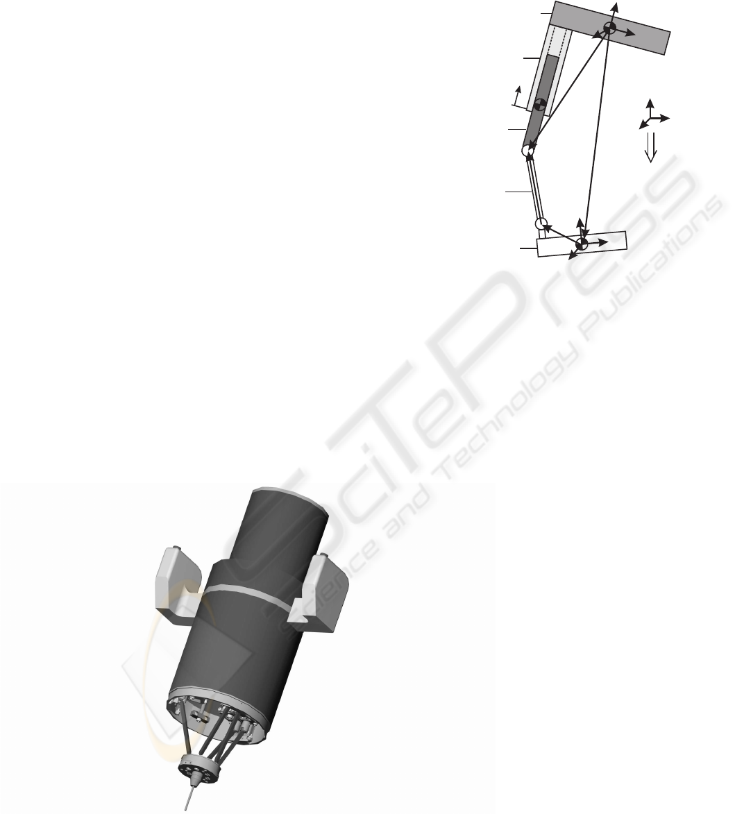
The mechanical device designed is a parallel robot
with six base-fixed actuators. The CAD model of
the surgical robot ITDII (Intelligent Tool Drive II) is
shown in Fig. 1. The robot base has six fixed linear
motors, i.e. the electrical part of the motors. Further-
more, there are guide rails, housing, and handles for
the hand-held operation, building together the robot
base. The sliders of the linear motors are connected
to the tool platform via six lightweight struts. At the
tool platform and at the sliders the struts are mounted
with spherical joints.
Because the base of the robot can be moved freely
Figure 1: Hand-held surgical robot ITDII - CAD model.
B
s,i
r
B
st,i
r
T
t,i
r
B
T
r
g
z
q
i
z
z
z
x
x
x
y
y
y
B
T
R
{W}
{T}
{B},{B }’
tool
platform
baseplatform
actuatori
slideri
struti
Figure 2: Topology of the parallel robot with fixed actua-
tors.
in space, adequate coordinate systems have to be de-
fined. For the calculation of the kinematic equations
four coordinate frames are considered (Fig. 2): (1)
the world (earth) frame {W}, (2) the tool frame {T}
in the tool’s centre of gravity, (3) the movable base
frame {B} in the base’s center of gravity, and (4) the
instantaneously coincident base frame {B’}, which is
fixed in {W}. The frame {B’} and the frame {B} are
aligned, if the base stands still. Without loss of gen-
erality the motion of both platforms is represented in
the {B’} frame, which reduces the complexity of the
kinematic description. The choice of the coordinates
has no influence on the value of the inertial forces.
For simplicity the gravity is calculated in the world
frame. Afterwards, the resulting force can be trans-
formed into the {B’} frame with little effort.
The pose of the tool is defined by the position
vector
B
r
T
and the orientation matrix
B
T
R in the {B}
frame, which build together the pose vector
B
X
T
=
(
B
r
T
,
B
T
R). From the matrix
B
T
R the fixed zyx-Euler
angles φ, θ, and ψ can be derived. The positions of
the tool joints
T
r
t,i
in the tool frame and the initial po-
sitions of the slider joints
B
r
s
0
,i
in the base frame for
each actuator i are known from the geometry of the
construction. The sliders actual positions
B
r
s,i
move
in z-direction of the base according to the guidance,
if the tool changes its position. Therefore, the initial
positions
B
r
s,i,x
=
B
r
s
0
,i,x
and
B
r
s,i,y
=
B
r
s
0
,i,y
in the
x-direction respectively the y-direction are not alter-
nated. The struts have the lengths l
i
.
DISTURBANCE FEED FORWARD CONTROL OF A HANDHELD PARALLEL ROBOT
45

3 MODELLING
For the model-based control of the robot, the non-
linear inverse dynamic description is required, espe-
cially if both platforms can be moved freely in the
entire workspace.
3.1 Inverse Kinematics
The inverse kinematics of the robot describes the non-
linear relationship between the relative tool-base pose
and the slider positions, which states the operating
point of the robot in the instantaneously coincident
base frame {B’}. Furthermore, the velocities and ac-
celerations of the sliders are given from the relative
motion of the tool and the base in {B’}.
3.1.1 Pose
Since the slider positions are constrained by the six
struts i = 1..6, the joint x and y distances between
slider and strut joints are given by
B
r
st,i,x
=
B
r
s,i,x
−
B
r
t,i,x
(1)
and
B
r
st,i,y
=
B
r
s,i,y
−
B
r
t,i,y
. (2)
With the assumption of constant strut lengths l
i
the
z-component of the joint distance vectors can be cal-
culated as
B
r
st,i,z
=
q
l
2
i
− (
B
r
st,i,x
)
2
− (
B
r
st,i,y
)
2
(3)
and the slider joint positions yield
B
r
s,i,z
=
B
r
t,i,z
+
B
r
st,i,z
. (4)
The required shift of the actuator positions with re-
spect of the starting positions
B
r
s
0
,i,z
is
q
i
=
B
r
s,i,z
−
B
r
s
0
,i,z
, (5)
which is measured by local positioning sensors.
3.1.2 Velocity
The generalized tool and base velocities
B
′
˙
X
T
= (
B
′
v
T
,
B
′
ω
T
) and
B
′
˙
X
B
= (
B
′
v
B
,
B
′
ω
B
) em-
brace the translational velocities
B
′
v
T
respectively
B
′
v
B
and the angular velocities
B
′
ω
T
and
B
′
ω
B
of both
rigid bodies. According to a rigid body motion the
tool joint positions and the base-fixed initial slider
joint positions can be determined from the general-
ized velocities. Due to the constant strut lengths, the
z-components of the relative slider velocities
B
′
v
st,i,z
= −
B
r
st,i,x
B
r
st,i,z
B
′
v
st,i,x
−
B
r
st,i,y
B
r
st,i,z
B
′
v
st,i,y
(6)
result from the constraint movement on a sphere with
radius l
i
. The relative velocities of the sliders, which
can be measured and controlled on the actuator level,
is
˙q
i
=
B
′
v
st,i,z
+
B
′
v
t,i,z
−
B
′
v
′
s,i,z
(7)
with the tool joint velocities
B
′
v
t,i,z
and the velocities
of the initial joint positions
B
′
v
′
s,i,z
.
3.1.3 Acceleration
Corresponding to the velocity derivation, the gener-
alized accelerations of the tool and the base are de-
fined by
B
′
¨
X
T
= (
B
′
a
T
,
B
′
α
T
) and
B
′
¨
X
B
= (
B
′
a
B
,
B
′
α
B
)
with the translational accelerations
B
′
a
T
and
B
′
a
B
and
the angular accelerations
B
′
α
T
and
B
′
α
B
. The acceler-
ations of the joints are assemblies of three terms: (1)
inertial acceleration a
′
, 2) centripetal acceleration a
′′
,
and (3) Coriolis acceleration a
′′′
. The inertial terms of
the slider joints are
B
′
a
′
s,i
=
B
′
a
B
+
B
′
α
B
×
B
r
s,i
, (8)
and the centripetal accelerations are
B
′
a
′′
s,i
=
B
′
ω
B
×
B
′
ω
B
×
B
r
s,i
. (9)
The Coriolis acceleration terms are non-zero in x-
direction
B
′
a
′′′
s,i,x
= 2·
B
′
ω
B,y
· ˙q
i
(10)
and in y-direction
B
′
a
′′′
s,i,y
= − 2·
B
′
ω
B,x
· ˙q
i
. (11)
The z-component
B
′
a
′′′
s,i,z
is identical zero.
Summarizing the three terms, the slider joint ac-
celerations in x and y direction result in
B
′
a
s,i,x
=
B
′
a
′
s,i,x
+
B
′
a
′′
s,i,x
+
B
′
a
′′′
s,i,x
(12)
B
′
a
s,i,y
=
B
′
a
′
s,i,y
+
B
′
a
′′
s,i,y
+
B
′
a
′′′
s,i,y
. (13)
The slider acceleration in z-direction is not a simple
sum, because the slider motion is constrained by the
struts according to the sphere equation
B
′
a
st,i,z
= −
B
r
st,i,x
B
r
st,i,z
B
′
a
st,i,x
+
B
′
a
nst,i,x
−
B
r
st,i,y
B
r
st,i,z
B
′
a
st,i,y
+
B
′
a
nst,i,y
−
B
′
a
nst,i,z
(14)
with the normal acceleration
B
′
a
nst,i
= −
B
r
st,i
×
B
′
v
st,i
×
B
′
v
st,i
/
B
r
st,i
2
(15)
Finally, the slider joint accelerations are
B
′
a
s,i,z
=
B
′
a
st,i,z
+
B
′
a
t,i,z
. (16)
ICINCO 2007 - International Conference on Informatics in Control, Automation and Robotics
46

and the acceleration of a slider’s center of gravity
yields
B
′
a
cg,i,z
=
B
′
a
s,i,z
+
B
′
ω
B
×
B
′
ω
B
×
B
r
scg,i
(17)
with the position offset
B
r
scg,i
between the slider joint
position and the slider’s centre of gravity.
3.2 Inverse Dynamics
The inverse dynamics of the robot describes the actu-
ator forces needed to move the tool’s centre of gravity
with a desired velocity and acceleration. Additionally,
the actuator forces are derived to stabilize the tool, if
the base is disturbed. In this section a brief sketch of
the ITDII robot’s inverse dynamics is given. A more
detailed description can be found in (Wagner et al.,
2006).
The rigid body dynamics of a parallel robot can be
described generally by the equation of motion
B
′
Λ
T
= M(q) ·
¨
q+ C(q,
˙
q) ·
˙
q+ G(q). (18)
with the generalized force
B
′
Λ
T
, which is necessary to
move the tool platform in a fixed frame {B’}. Within
this equation M is the generalized mass matrix, C is
the centripedal and Coriolis component and G is the
gravity component of the platform. These parameters
depend on the operationg point of the robot. The gen-
eralized force is converted into actuator forces using
the Jacobian matrix of the robot. Additionally, the in-
ertia forces
F
s,i
= m
s,i
h
B
′
a
cg,i,z
−
B
W
Rg
z
i
. (19)
are taken into acount with the slider masses m
s,i
. The
gravitiy vector g = (0 0 − 9, 81m/s
2
)
T
can be trans-
formed from the {W} frame into the {B} frame using
the rotation matrix
B
W
R. Since the major part of the
strut masses is concentrated in the joints and since the
link beetween the joints is lightweight, the struts can
be separated into two parts, which can be added to the
slider and tool components (Honegger, 1999). Corre-
spondingly the strut masses and inertias are not con-
sidered in the inverse dynamics explicitly. In a first
attempt the friction forces are neglected as well. The
latter can easily be extended on the actuator level, if
necessary. The non-working reaction forces/torques
of the actuators are perpendicular to the actuator mo-
tions and, therefore, not considered in the robot dy-
namics.
For the calculation of all force components the rel-
ative velocity and acceleration between the tool and
the base as well as the absolute orientation of the robot
in the world coordinates must be available. It should
be mentioned, that the actuator forces are not simple
vector sums of the tool and the base related forces,
since the equation of motion is non-linear. However,
if the tool is fixed, the
B
′
Λ
T
term vanishes and the re-
maining forces for the slider mass acceleration yields
a quite simple form (19).
4 CONTROL STRUCTURE
The robot control must be suited to adjust the tool
against a movable workpiece and to decouple the tool
from disturbances at the base. Therefore, a control
structure was designed, which combines a servo con-
trol on the local axis level with a disturbance feed-
forward control in the global Cartesian space (Fig. 3).
For the controller design the adequate choice of
co-ordinate systems is essential, since the complete
robot can be moved freely in space and the component
inertia forces are related to a earth fixed (respectively
inertia) reference system. The local stabilization is
based on the robot kinematics, which describes the
relative pose between tool and base in relation to the
actuator positions. Here, the actuator position are not
dependent on the tool and base reference. In contrast,
the feed-forward control uses the inverse dynamics
block, which is definded in {B’}. The sensor sig-
nals for the base pose, velocity and acceleration are
retrieved in the world frame. Furthermore, the de-
sired tool motion is given in the world frame as well.
Therefore, the tool and base motion signal are con-
verted to {B’} co-ordinates before they are applied to
the inverse kinematics. This geometric transforma-
tion can be done with little effort.
The local control is based on the slider position
and velocity sensor signals q and
˙
q. The actuator sig-
nals are compared to the desired actuator signals q
d
and
˙
q
d
. Using the generalized tool mass matrix M a
PD-controller generates the force signals F
fb
needed
to stabilize the tool. The reference signals q
d
and
˙
q
d
result from the desired tool signals
W
X
Td
, and
W
˙
X
Td
and from the actual base coordinates
W
X
B
, and
W
˙
X
B
both in Cartesian world coordinates, using the inverse
kinematics of the parallel robot.
The feed-forward control block consists of two
inputs, the tool reference signals
W
X
Td
,
W
˙
X
Td
, and
W
¨
X
Td
and the actual base signals
W
X
B
,
W
˙
X
B
, and
W
¨
X
B
. Using the inverse dynamic model the feed-
forward forces F
ff
are calculated which are required
to move the tool as desired, while the disturbances
from the base are canceled. If the inverse dynamic
model and the sensor/actuator signals are assumed to
be perfect, the local control error will be zero. How-
ever, the inverse model is not really complete due to
the neglected strut masses, actuator friction and un-
DISTURBANCE FEED FORWARD CONTROL OF A HANDHELD PARALLEL ROBOT
47
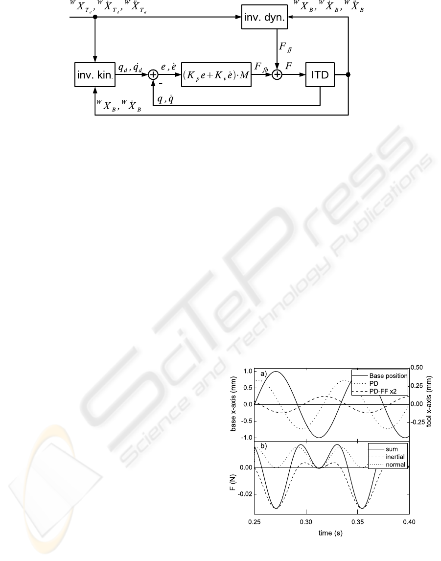
Figure 3: Control structure; local servo loop and global disturbance feed forward control.
measured disturbances. These model uncertainties
are compensated by the local pose control. The pre-
sented structure is not a classical cascaded structure,
because the base coordinates are not influenced im-
mediately by the control action. The base motion re-
sults from the disturbance forces of the human opera-
tor. That means that no feed-back from the actuators
to the base motion is assumed due to the large base
mass and that the sensing of the base motion serves
for the referencing of coordinates only.
In the realized system it is necessary to measure
the pose, the velocity and the acceleration of the base.
The tool coordinates are calculated from the desired
tool trajectory. To take care of force feed-back dur-
ing the processing of the workpiece, additional sen-
sors measuring the tool motion or forces could be im-
plemented in a feed-back control. This may make
sense in special cases. However, backlash effects in
the joints could lead to a destabilization of the con-
trolled system. Therefore, and for the sake of sim-
plicity we are content with the local stabilization.
As shown in literature (Riebe and Ulbrich, 2003),
a friction compensation is essential in the real appli-
cation, which can be added on the local axis level. To
separate the kinetic effects from the friction effects,
such a compensation is neglected in this paper. The
control structure has been implemented in the simula-
tion environment Matlab/Simulink using a fixed sam-
pling time of 1 ms. As a consequence the minimum
delay in the control loop is 1 ms as well. The forward
dynamics of the robot ITD used in the closed loop
simulations has been modelled with the SimMechan-
ics toolbox.
5 SIMULATION
The simulations presented in this section mainly sup-
port the description of the disturbance decoupling
ability of the system. Additionally, the overall tra-
jectory tracking quality is described at the end using
a standard circle test (ballbar-test).
5.1 Tool Stabilization
The first simulations describe the system disturbance
response in the frequency domain. In the first sim-
ulations the control parameters are configured for a
critically damped PD control loop with a system fre-
quency Ω = 60Hz. Figure 4(a) shows the tool motion
after application of a 12 Hz, 1 mm sinusoidal signal
at the base. The straight line represents the stimu-
lus in the x-direction, which can be referenced to the
left hand scale. The amplitude of the tool position re-
sponse using a PD control (dotted line) and using a
PD control with additional feed forward disturbance
Figure 4: Response on a 12 Hz, 1 mm sinusoidal trans-
lational base disturbance in x-axis; (a) base position stim-
ulus (straight line, left-hand scale), tool position response
(PD control, dotted line, right-hand scale), tool position re-
sponse multiplied by a factor of two (PD control with distur-
bance feed-forward, dotted line, right-hand scale); (b) Force
needed for feed-forward compensation.
ICINCO 2007 - International Conference on Informatics in Control, Automation and Robotics
48
compensation (dashed line) can be extracted from the
right hand scale. For a better readability the later is
multiplied by a factor of two.
As a result the PD controlled tool is damped
against the base disturbance with a transfer factor of
0.3 (-10dB) due to its limited bandwidth. Adding the
feed-forward control the transfer factor decreases to
0.06 (-24dB).
The actuator force needed to cancel the distur-
bances is plotted in Fig. 4(b) for the first actuator. The
resulting force F (straight line) is the total of all force
components. The inertial component (dashed line) re-
sults from the tool and the slider acceleration (8) and
the normal component (dotted line) is a consequence
of the strut rotation velocity (6). No Coriolis or cen-
tripedal forces are generated for a translational tool
movement. While the tool-pose reaction seams to be
more or less a sinusoidal function, higher harmonic
distortions are noticeable in the inertial component.
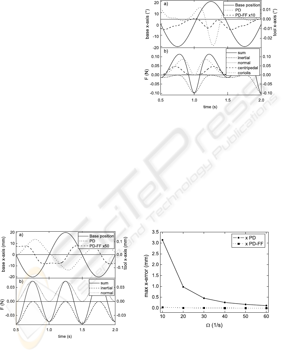
Now, the sinusoidal stimulus is shifted to 1 Hz and
20 mm amplitude (Fig. 5) compared to Fig. 4. Here,
the feed-forward related position response is multi-
plied by a factor of 50. As a result of the lower fre-
quency the PD-loop has an increased damping effect
with a transfer factor of 6 · 10
−3
(-45dB) respectively
6.5· 10
−5
(-84dB) with feed forward control (Fig. 5).
The pose response signal in the large signal case is
not a sinusoidal signal anymore due to the non-linear
coupling between tool and base.
A sinusoidal stimulation of the base orientation
Figure 5: Response on a 1 Hz, 20 mm sinusoidal trans-
lational base disturbance in x-axis; (a) base position stim-
ulus (straight line, left-hand scale), tool position response
(PD control, dotted line, right-hand scale), tool position re-
sponse multiplied by a factor of 50 (PD control with distur-
bance feed-forward, dotted line, right-hand scale); (b) Force
needed for feed-forward compensation.
Figure 6: Response on a 1 Hz, 20
o
sinusoidal rotational base
disturbance around the x-axis; (a) base orientation stimu-
lus (straight line, left-hand scale), tool orientation response
(PD control, dotted line, right-hand scale), tool orientation
response multiplied by a factor 10 (PD control with distur-
bance feed-forward, dotted line, right-hand scale); (b) Force
needed for feed-forward compensation.
around the x-axis and its response is shown in Fig.
6(a). The forces needed to stabilize the tool are plot-
ted in Fig. 6(b). Here, the Coriolis (large dotted line)
and centripedal (large dashed line) forces are in the
range of the inertia forces. Unlike an intuitive estima-
tion the Coriolis and centripedal components cannot
be neglected in this special robot application.
Figure 7: x- axis response on a 1 Hz, 20 mm sinusoidal
translational base disturbance in dependence on the servo
loop frequency.
The decoupling behaviour from the base motion
strongly depends on the choice of the parameter Ω
and the delay in the feed-back loop, which is at least
one sampling period. This is shown in Fig.7 and Fig.8
DISTURBANCE FEED FORWARD CONTROL OF A HANDHELD PARALLEL ROBOT
49
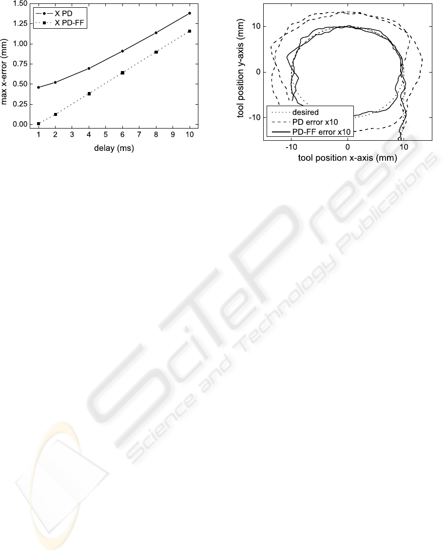
Figure 8: x- axis response on a 1 Hz, 20 mm sinusoidal
translational base disturbance in dependence on the sensor
delay.
for a base disturbance of 1 Hz and 1 mm.
The pose error amplitude and phase decrease with
increasing control loop frequency. With disturbance
feed forward control the error is generally smaller,
however the quality strongly depends on the sensor
delay. To estimate the limit time lack that can be al-
lowed the pose error is plotted against the sensing de-
lay. For instance, the delay should not exceed 3 ms,
if a pose accuracy of 0.3 mm is required. (Certainly,
additional error sources must be considered).
5.2 Tracking Control
To assess the possibilities of the disturbance feed for-
ward control the standard circle (ballbar) test was sim-
ulated assuming an additional white Gaussian sen-
sor noise with a translational standard deviation of
σ
accel
= 0.17mm/s
2
and a rotational standard devia-
tion of σ
rot
= 0.17rad/s for all axes. Figure 9 shows
the reference trajectory, which has to be followed with
a velocity of 0.1 m/s, and the actual trajectories using
a PD control and using a PD control with disturbance
feed forward. The deviation from the reference tra-
jectory is exaggerated by a factor of five. The mean
pose error are 0.35 mm and 0.10 mm with respectively
without feed forward control. The standard deviations
are 0.051 mm and 0.052 mm. Also for the reference
action the feed forward control diminishes the pose
error remarkably. Because the signal noise from the
base sensors is injected into the inverse kinematics
block as well as into the inverse dynamics block, it in-
fluences the PD control loop once and the PD control
with feed forward control twice. However, the persis-
tent pose noise is not much larger with a feed forward
control compared to the pure PD control approach.
Figure 9: Standard circle test with white Gaussian sensor
noise; σ
accel
= 0.17mm/s
2
translational standard deviation,
σ
rot
= 0.17rad/s rotational standard deviation, v = 0.1m/s
feed speed.
6 DISCUSSION
The simulations show, that if a complete model of the
parallel robot and adequate sensor signals are avail-
able, a feed forward control can lead to a decoupling
from base disturbances with high damping factors.
For the quality of the decoupling the sensor noise and
the sensor delay are essential. The simulated damp-
ing value of 6.5 · 10
−5
in the 1 Hz case (Fig. 5) must
be interpreted with care, because the quality of the
decoupling is influenced by numerical errors in this
range. Furthermore, model uncertainties and sensor
errors do not allow such a high precision in real-world
applications. Within the control approach the base
pose, velocity and acceleration must be measured or
observed accurately in the inertia system. This is a
serious problem, because not only sensor latency and
noise must be considered but also misalignment, bias,
drift, etc..
For the simulations an ideal model is assumed
without geometric or parametric errors and without
considering the friction in the actuators and joints.
An enhancement of the dynamic model can be done
with acceptable effort, e.g. the modelling of friction
on the actuator level. However, the quantity of fric-
tion and its influence on the dynamics depends on
the special mechanical implementation and many pa-
rameters. Therefore a possible model extension must
be considered if the robot is realized. In contrast to
the intuitive impression that for the size, mass and
dynamics of a hand-held robot the Coriolis and cen-
tripedal forces do not play any role, the simulations
show that these force components make a remarkable
ICINCO 2007 - International Conference on Informatics in Control, Automation and Robotics
50

contribution to the total force in the actuators. Thus,
a simplification of the model by neglecting the veloc-
ity related force components is not suitable. Finally,
the simulations show in which range of precision a
feed forward control does improve the decoupling be-
haviour and in which range the feed forward control
can be neglected.
7 CONCLUSION
A model-based approach is presented to control the
tool pose of a handheld robot and to decouple the tool
from base disturbances. An adequate definition of co-
ordinate frames for the dynamics modelling and the
controller design reduces the effort for the implemen-
tation. The feasibility of a feed-back control on the lo-
cal axis level in combination with a disturbance feed
forward control on the robot level in world coordi-
nates is shown. The local control is able to stabilize
the robot and to avoid huge errors due to model un-
certainties and disturbances. The feed forward control
ensures the free movement of the robot in space, while
measured disturbances can be compensated for. Fur-
thermore, the usage of a non-linear inverse dynamics
model enables the precise disturbance feed-forward
control under different operational conditions. For the
feed-forward control sensor error and delay are cru-
cial.
REFERENCES
Chen, Y. and McInroy, J. E. (2004). Decoupled control of
flexure-jointed hexapods using estimated joint-space
mass-inertia matrix. IEEE Transactions on Control
Systems Technology, 12.
Honegger, M. (1999). Konzept einer Steuerung mit adap-
tiver nichtlinearer Regelung f
¨
ur einen Parallelma-
nipulator. Dissertation, ETH Zurich, Switzerland,
http://www.e-collection.ethbib.ethz.ch.
Honegger, M., Codourey, A., and Burdet, E. (1997). Adap-
tive control of the hexaglide, a 6 dof parallel manipu-
lator. IEEE International Conference on Robotics and
Automation, Albuquerque, USA.
Huynh, P. (2001). Kinematic performance comparison of
linar type parallel mechanisms, application to the de-
sign and control of a hexaslide. 5th International con-
ference on mechatronics technology (ICMT2001), Sin-
gapore.
Koekebakker, S., Teerhuis, P., and v.d. Weiden, A. (1998).
Multiple level control of a hydraulically driven flight
simulator motion system. CESA Conference, Ham-
mammet.
Merlet, J. (2000). Parallel robots. Kluwer Academic Pub-
lisher, Dordrecht, Netherlands.
Pott, P., Wagner, A., K
¨
opfle, A., Badreddin, E., M
¨
anner,
R., Weiser, P., Scharf, H.-P., and Schwarz, M. (2004).
A handheld surgical manipulator: Itd - design and first
results. CARS 2004 Computer Assisted Radiology and
Surgery, Chicago, USA.
Riebe, S. and Ulbrich, H. (2003). Modelling and online
computation of the dynamics of a parallel kinematic
with six degrees-of-freedom. Archive of Applied Me-
chanics, 72:817–829.
Stewart, D. (1965-1966). A platform with six degrees of
freedom. Proceedings of the Institute of Mechanical
Engineering, 180:371–386.
Takanokura, M. and Sakamoto, K. (2001). Physiological
tremor of the upper limb segments. Eur. J. Appl. Phys-
iol., 85:214–225.
T
¨
onshoff, H., Grendel, H., and Grotjahn, M. (2002). Mod-
elling and control of a linear direct driven hexapod.
Proceedings of the 3rd Chemnitz Parallel Kinemat-
ics Seminar PKS 2002, 2002 Parallel Kinematic Ma-
chines Int.Conf.
Wagner, A., Pott, P., Schwarz, M., Scharf, H.-P., Weiser,
P., K
¨
opfle, A., M
¨
anner, R., and Badreddin, E.
(2004). Control of a handheld robot for orthopedic
surgery. 3rd IFAC Symposium on Mechatronic Sys-
tems, September 6-8, Sydney, Australia, page 499.
Wagner, A., Pott, P., Schwarz, M., Scharf, H.-P., Weiser, P.,
K
¨
opfle, A., M
¨
anner, R., and Badreddin, E. (2006). Ef-
ficient inverse dynamics of a parallel robot with two
movable platforms. 4rd IFAC Symposium on Mecha-
tronic Systems, Heidelberg, Germany.
DISTURBANCE FEED FORWARD CONTROL OF A HANDHELD PARALLEL ROBOT
51
