
REAL-TIME INTER- AND INTRA- CAMERA COLOR MODELING
AND CALIBRATION FOR RESOURCE CONSTRAINED ROBOTIC
PLATFORMS
Walter Nistic
`
o and Matthias Hebbel
Robotics Research Institute (IRF), Universit
¨
at Dortmund, Otto-Hahn-Str. 8, Dortmund, Germany
Keywords:
Camera modeling, color correction, evolutionary algorithms, real time.
Abstract:
This paper presents an approach to correct chromatic distortion within an image (vignetting) and to compensate
for color response differences among similar cameras which equip a team of robots, based on Evolutionary
Algorithms. Our black-box approach does not make assumptions concerning the physical/geometrical roots
of the distortion, and the efficient implementation is suitable for real time applications on resource constrained
platforms.
1 INTRODUCTION
Robots which base their perception exclusively on vi-
sion, without the help of active sensors such as laser
scanners or sonars, have to deal with severe additional
constraints compared to generic computer vision ap-
plications. The robots have to interact with a dynamic
(and sometimes even competitive or hostile) environ-
ment and must be able to take decisions and react to
unforeseen situations in a fraction of a second, thus
the perception process has to run in real-time with
precise time boundaries. In particular, autonomous
robots are typically constrained even in terms of com-
putational resources, due to limitations in power sup-
ply, size, and cost. A very popular approach espe-
cially for indoor environments is color-based image
segmentation, and even though dynamic approaches
have been demonstrated (for example, (Iocchi, 2007)
(Schulz and Fox, 2004)), static color classification
(Bruce et al., 2000) is still the most widely used solu-
tion, due to its efficiency and simplicity. In a group of
homogeneous robots, which make use of color infor-
mation in their vision system, it is important that all
cameras produce similar images when observing the
same scene, to avoid to have to individually calibrate
the vision system of each robot, a procedure which is
both time consuming and error prone. Unfortunately,
even when the cameras are from the same model and
produced from the same manufacturer, such assump-
tion does not always hold (R
¨
ofer, 2004).
1.1 The Platform
This work has been developed on the popular Sony
Aibo ERS-7 robot (Sony Corporation, 2004), which is
the only complete standard platform widely adopted
for robotic applications to date. The robot is equipped
with a 576MHz 64bit RISC CPU, 64MB of main
memory, and a low-power CMOS camera sensor with
a maximum resolution of 416 × 320 pixel. Images
are affected by a ring-shaped dark blue cast on the
corners, and different specimen of the same model
tend to produce slightly different color responses to
the same objects and scene. Our experiments have
been conducted using the YUV color space which is
natively provided by most common cameras, but the
approach can be applied unaltered to the RGB color
space. The Aibo production has been recently discon-
tinued by Sony, but several new commercially avail-
able robotic kits are being introduced on the market,
with similar characteristics in terms of size and power,
often equipped with embedded RISC CPUs or PDAs
and low quality compact flash cameras.
1.2 Related Work
Whenever object recognition is mostly based on color
classification, the dark / colored cast on the corners of
378
Nisticò W. and Hebbel M. (2007).
REAL-TIME INTER- AND INTRA- CAMERA COLOR MODELING AND CALIBRATION FOR RESOURCE CONSTRAINED ROBOTIC PLATFORMS.
In Proceedings of the Fourth International Conference on Informatics in Control, Automation and Robotics, pages 378-383
DOI: 10.5220/0001631403780383
Copyright
c
SciTePress
the images captured by the on board camera is a se-
rious hindrance. Vignetting is a radial drop of image
brightness caused by partial obstruction of light from
the object space to image space, and is usually de-
pendent on the lens aperture size (Nanda and Cutler,
2001) (Kang and Weiss, 2000). These approaches, as
well as (Manders et al., 2004), treat the problem in
terms of its physical origins due to geometrical de-
fects in the optics, and are mostly focused on radio-
metric calibration, i.e. ensuring that the camera re-
sponse to illumination after the calibration conforms
to the principles of homogeneity and superposition.
However, none of the proposed methods deals with
chromatic distortion, as is the case of our reference
platform, and other inexpensive low power CMOS
sensors. Recently, a few papers have attempted to
tackle such problem. These solutions share a simi-
lar approach to minimize the computational costs by
using lookup tables to perform the correction in real
time, while the expensive calibration of the correc-
tion tables is performed off-line. In (Xu, 2004) the
author uses a model based on a parabolic lens geom-
etry, solved through the use of an electric field ap-
proach. No quantitative analysis of the results is pro-
vided, but this technique has been successfully used
in practice by one team of autonomous robots in the
RoboCup Four-Legged League.
1
Another success-
ful technique used in RoboCup has been presented in
(Nistic
`
o and R
¨
ofer, 2006), based on a purely black-
box approach where a polynomial correction function
is estimated from sample images using least square
optimization techniques. Since this approach does not
rely on assumptions concerning the physics of the op-
tical system, we feel that it can be more effective in
dealing with digital distortions such as saturation ef-
fects. Again no quantitative analysis has been pre-
sented, and both papers do not address the problem of
inter-robot camera calibration, which has been treated
in (Lam, 2004) with a simple linear transformation of
the color components considered independently.
2 COLOR MODEL
The first step to understand the characteristics of this
chromatic distortion, was to capture images of special
cards that we printed with uniform colors, illuminat-
ing them with a light as uniform as possible, trying
to avoid shadows and highlights.
2
Then we calcu-
1
RoboCup is an international joint project to promote
AI, robotics, and related fields. http://www.robocup.org/
2
However, this is not so critical, and the use of a profes-
sional diffuse illuminator is not necessary, as our approach
can deal well with noise and disturbances (see Section 2.1).
lated the histograms of the three image spectra, with
a number of bins equal to the number of possible val-
ues that each spectrum can assume, i.e. 256. Under
these conditions, the histograms of such uniform im-
ages should be uni-modal and exhibit a very narrow
distribution around the mode (in the ideal case, such
distribution should have zero variance, i.e. all the pix-
els have exactly the same color) due only to random
noise. Instead, it could be observed that the variance
of the distribution is a function of the color itself; in
case of the U channel, it appears very narrow for cold
/ bluish color cards, and very wide for warm / yel-
lowish cards (Figure 1(a)). Consequently, we model
the chromatic distortion d
i
for a given spectrum i of a
given color I as a function of I
i
itself, which here we
will call brightness component λ
i
(I
i
).
(a) (b)
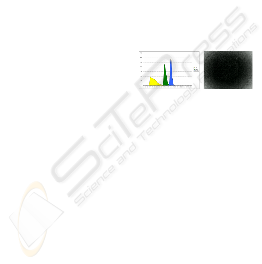
Figure 1: a) Histograms of the U color band for uniformly
colored images: yellow, green and skyblue. Notice how the
dispersion (due to the vignetting) increases inverse propor-
tionally to the position of the mode. b) Brightness distri-
bution of the U color band for a uniformly yellow colored
image.
The distribution itself is not centered around the
mode, but tends to concentrate mostly on one side
of it. The reason for this becomes apparent by ob-
serving the spatial distribution of the error (cf. Fig-
ure 1(b)); the phenomenon itself is nothing but a ring
shaped blue/dark cast, whose intensity increases pro-
portionally to the distance from the center of the dis-
tortion (u
d
, v
d
), which lies approximately around the
optical center of the image, the principal point. So,
let r =
p
(x − u
d
)
2
+ (y − v
d
)
2
, then we define
the radial component as ρ
i
(r(x, y)). Putting together
brightness and radial components, we obtain our dis-
tortion model:
d
i
(I(x, y)) ∝ ρ
i
(r(x, y)) · λ
i
(I
i
(x, y)) (1)
Now, due to the difficulty to analytically derive
ρ
i
, λ
i
, ∀i ∈ {Y, U, V } about which little is known,
we decided to use a black-box optimization ap-
proach. Both sets of functions are non-linear, and we
chose to approximate them with polynomial functions
REAL-TIME INTER- AND INTRA- CAMERA COLOR MODELING AND CALIBRATION FOR RESOURCE
CONSTRAINED ROBOTIC PLATFORMS
379

(McLaurin series expansion).
ρ
i
(r) =
n
P
j=0
%
i,j
· r
j
λ
i
(I
i
) =
m
P
j=0
l
i,j
· I
j
i
(2)
The unknown polynomial coefficients %
i,j
and l
i,j
can
be estimated, from a set of samples, using naturally
inspired machine learning techniques. So, the final
vignetting correction function is as follows:
I
0
i
(x, y) = I
i
(x, y) − ρ
i
(r(x, y)) · λ
i
(I
i
(x, y)) (3)
where I
0
i
(x, y) is the corrected value of the spectrum
i of the given pixel.
2.1 Reference Color Estimation
To be able to model our error functions, we must
first estimate how the pictures should look like, if
they were not affected by any chromatic distortion.
Since most of the image area exhibits little to no dis-
tortion, we define as reference color of a single im-
age the most frequent color appearing in its spec-
tra. So we calculate the histograms of the 3 color
spectra (number of bins = number of color levels =
256) and we find the modes ¯r
Y
i
, ¯r
U
i
, ¯r
V
i
, which repre-
sent the reference color for image i. However, a sin-
gle image can be affected by other sources of noise,
such as a temporary change of light intensity, strob-
ing (aliasing between the camera shutter speed and
the light source power frequency, which affects flu-
orescent lights) or shadows: consequently, the his-
tograms’ modes might have temporary fluctuations,
or exhibit multiple nearby modes. To make our sys-
tem more robust toward this kind of noise, we col-
lect multiple pictures of each colored cards in a log
file, and we partition the images therein contained
into image classes
3
, where a class represents a cer-
tain color card (e.g. yellow, orange, green, blue) at
a certain light intensity and camera settings. For each
image class j we want to have a single reference color
¯
R
Y
j
,
¯
R
U
j
,
¯
R
V
j
: of course this could be obtained by av-
eraging the references from all the images which be-
long to the class, but this would still be affected by
outliers. Instead, we track the current reference of a
given class using a simple first order linear Kalman
filter (Welch and Bishop, 2003):
• For each image i in the log, a reference value is es-
timated for the 3 spectra ¯r
Y
i
, ¯r
U
i
, ¯r
V
i
, as the modal
value of the corresponding histogram
3
With image class or color class here we will refer to
a color card captured under certain lighting settings, i.e.
the same color card can be represented by different color
classes, like blue-dark and blue-light.
• Constant value process model: the predicted ref-
erence color
ˆ
R
Y
j
,
ˆ
R
U
j
,
ˆ
R
V
j
for class j at the fol-
lowing step (image i) remains the same as the one
after the measurement update of image i − 1
• We use the output of the Kalman filter to perform
the partitioning into color classes on the fly; a new
class is generated when:
∃c ∈ {Y, U, V } :
ˆ
R
c
j
− ¯r
c
i
> ϑ (4)
where ϑ is a confidence threshold; so if at least
one of the spectra in the reference of the current
image differs too much from the expected refer-
ence for the current class, then we need to create
a new color class. A new class reference is initial-
ized to the value extracted from the current image.
• Measurement model: we update the running class
reference
ˆ
R
Y
j
,
ˆ
R
U
j
,
ˆ
R
V
j
using the reference ex-
tracted from the current image
2.2 Inter-camera Model
In the general case, it is possible that to completely
correct the difference in color response between two
cameras it is necessary to rotate the color space of one
camera to align with the other. This however, is not
feasible for a real time implementation for robotic ap-
plications. To capture the dependencies between the
3 color components and the distance from the image
center, we would need a 256
3
· ρ
max
look-up table,
which would have a size of over 2GB even for our
low resolution camera. Otherwise, we could perform
the rotation with the multiplication of a 3 × 3 ma-
trix by our color vector; since such costly operation
would have to be performed for every pixel, it would
slow down the image processing too much.
In (Lam, 2004) the author suggests a simple linear
transformation of the 3 color components of the cam-
era to be calibrated, treating them independently from
each other; such an approach is used in image pro-
cessing programs to perform adjustments in the color
temperature of a picture. Since we are going to use
an evolutionary approach to the optimization process,
we have decided to give more freedom to the inter-
camera transformation, by using higher order polyno-
mials instead:
I
00
i
(x, y) = A
i
(I
0
i
(x, y)) =
4
P
j=0
a
i,j
· (I
0
i
(x, y))
j
(5)
I
0
i
(x, y) is the i-th color component of pixel x, y of
the camera that we want to calibrate, a
i,j
are the
transformation coefficients which have to be learned,
and I
00
i
(x, y) is the resulting value, for a certain color
ICINCO 2007 - International Conference on Informatics in Control, Automation and Robotics
380

spectrum i ∈ {Y, U, V }, which should match the
color as it would appear if taken by the camera of the
reference (“alpha”) robot. Further, we must obtain I
0
i
from I
i
by applying the vignetting correction as de-
scribed. All robots in the team have to be calibrated
to match the color representation of the “alpha” robot,
hence each robot will have its own set of coefficients
a
i,j
.
When different cameras exhibit similar vignetting
characteristics, the vignetting correction polynomials
can be calculated only once for all cameras, then the
inter-camera calibration can be performed indepen-
dently and using much less sample images. In fact,
in our experiments we have seen that learning both
polynomial sets at the same time can easily lead to
over-fitting problems, with the inter-camera calibra-
tion polynomials which also end up contributing to
compensate the vignetting distortion (for example by
clipping the high and low components of the color
spectra), but this results in a poor generalization to
the colors which are out of the training set.
2.3 Realtime Execution
After optimizing off-line the parameters %
i,j
, l
i,j
, a
i,j
with the techniques presented in Section 3, we are
able to calculate the corrected pixel color values
(Y
00
, U
00
, V
00
), given the uncorrected ones (Y, U, V )
and the pixels’ position in the image (x, y). Perform-
ing the polynomial calculations for all the pixels in
an image is an extremely time-consuming operation,
but it can be efficiently implemented with Look-Up
Tables:
• radialLU T[x, y] =
p
(x − u
d
)
2
+ (y − v
d
)
2
stores the pre-computed values of the distance of
all the pixels in an image from the center of dis-
tortion (u
d
, v
d
);
• colorLU T [r, l, i] = A
i
(l − ρ
i
(r) · λ
i
(l)) where
r = radialLUT [x, y], l = I
i
(x, y) ∈ [0 . . . 255]
and i ∈ {Y, U, V } is the color spectrum. We fill
the table for all the possible values of r, l, c, the
size of the table is 256 · r
max
· 3 elements, so it
occupies only ≈ 200KBytes in our case
The look-up tables are filled when the robot is booted;
afterward it is possible to correct the color of a pixel
in real-time by performing just 2 look-up operations.
3 PARAMETER OPTIMIZATION
The goal is to find an “optimal” parameter set for the
described color model given a set of calibration im-
ages as previously described. Thus, we consider as
optimal the parameter set which minimizes the “func-
tion value” (from now on referred to as fitness), de-
fined as the sum of squared differences of the pixels
in an image from the reference value calculated for
the color class in which the image belongs. To calcu-
late the fitness of a certain parameter set, given a log
file of images of colored cards, we proceed as follows:
• For each image I
i,k
in the log file (i is the color
band, k the frame number), given its reference
value previously estimated R
i,k
, the current fit-
ness F
k
i
is calculated as:
F
k
i
=
X
(x,y )
I
00
i,k
(x, y) − R
i,k
2
(6)
• The total fitness F
i
is calculated as the sum of the
F
k
i
where each k is an image which belong to a
different color class; this to ensure that the final
parameters will perform well across a wide spec-
trum of colors and lighting situations, which oth-
erwise might only fit a very specific situation.
The optimization process is performed independently
for each color band i ∈ {Y, U, V }. To optimize the
vignetting correction, we use for A() (from Equation
5) the identity function, and the references R
i,k
which
are extracted from the same log (and same robot) that
we are using for the optimization process. In case
of inter-robot calibration instead, only A
i
() will be
optimized, ρ
i
(), λ
i
() will be fixed to the best func-
tions found to correct the vignetting effect, and the
references R
i,k
are extracted from a log file gener-
ated from another (“alpha”) robot, which is used as
reference for the calibration. If we want to opti-
mize the center of distortion (u
d
, v
d
), we need a set
of ρ
i
(), λ
i
() calculated in a previous evolution run
4
:
as fitness for this process we use the sum of the fit-
nesses of all 3 color channels, under the assumption
that there is only one center of distortion for all color
bands.
3.1 Simulated Annealing (SA)
In Simulated Annealing (Kirkpatrick et al., 1983) in
each step the current solution is replaced by a random
“nearby” solution, chosen with a probability that de-
pends on the corresponding function value (“Energy”)
and on the annealing temperature T . The current so-
lution can easily move “uphill” when T is high (thus
jumping out of local minima), but goes almost ex-
clusively “downhill” as T approaches zero. In our
work we have implemented SA as follows (Nistic
`
o
and R
¨
ofer, 2006).
4
Otherwise, changing u
d
, v
d
would have no effect on
the fitness
REAL-TIME INTER- AND INTRA- CAMERA COLOR MODELING AND CALIBRATION FOR RESOURCE
CONSTRAINED ROBOTIC PLATFORMS
381

In each step, the coefficients %
i,j
, l
i,j
(vignetting
reduction) or a
i,j
(inter-robot calibration) or (u
d
, v
d
)
(center of distortion) are “mutated” by the addition of
zero mean gaussian noise, the variance of which is
dependent on the order of the coefficients, such that
high order coefficients have increasingly smaller vari-
ances (decreasing order of magnitude) than low order
ones, following the idea that small changes in the high
order coefficients produce big changes in the overall
function. The mutated coefficients are used to correct
the image, as in Equation 5.
For each image I
i,k
in the log file (i is the color
spectrum, k the frame number), given its reference
value previously estimated R
i,k
, the current “energy”
E for the annealing process is calculated as in Equa-
tion 6. The “temperature” T of the annealing is low-
ered using a linear law, in a number of steps which
is given as a parameter to the algorithm to control
the amount of time spent in the optimization process.
The starting temperature is normalized relative to the
initial energy, so that repeating the annealing process
on already optimized parameters has still the possi-
bility to perform “uphill moves” and find other opti-
mum regions. The process ends when the tempera-
ture reaches zero; the best parameters found (lowest
energy) are retained as result of the optimization pro-
cess.
This approach has proved to work well with our
application, however it has 2 shortcomings:
• The search space is very irregular and has mul-
tiple local and even global optima. One reason
for the latter is that the function to be optimized
is the product of different terms (ρ
i
() · λ
i
()), so
that exactly the same result can be achieved by
multiplying one term by a factor and the other by
its reciprocal, or inverting the sign for both terms,
etc.
• The variances used to mutate the coefficients give
a strong bias to the final results, as it is not possi-
ble to fully explore such a wide search space in a
reasonable time; the depicted approach lacks the
ability to find “good” mutation parameters, apart
from the simple heuristic of decreasing the vari-
ance order at the increase of the coefficient order
Both issues can be dealt with efficiently by Evolution
Strategies.
3.2 Evolution Strategies (ES)
Evolution Strategies (Schwefel, 1995) use a parent
population of µ ≥ 1 individuals which generate
λ ≥ 1 offsprings by recombination and mutation.
ES with self-adaption additionally improve the con-
trol of the mutation strength: each parameter which
has to be optimized (object parameter) is associated
with its own mutation strength (strategy parameter).
These strategy parameters are also included in the en-
coding of each individual and are selected and inher-
ited together with the individual’s assignments for the
object parameters.
An offspring is created by recombination of the
parents. We use two parents to generate an offspring,
then such offsprings are subject to mutation.
The selection operator selects the parents for the
next generation based on their fitness. In case of the
(µ, λ)-strategy only the best µ individuals out of the
offsprings are chosen to be the parents of the next gen-
eration. Our implementation works similarly as the
annealing process, with the following exceptions:
• (µ, λ) strategy with self-adaption, the strategy pa-
rameters are initialized with the same sigmas used
in the annealing process;
• We terminate the evolution process when n gen-
erations have passed without any fitness improve-
ment
Having µ > 1 means that several different “optimal”
areas of the search space can be searched in parallel,
while the self-adaptation should make the result less
dependent from the initial mutation variances.
4 EXPERIMENTS AND RESULTS
At first we compared the two optimization techniques
to see what is most suitable for our application. We
ran the optimization on a log file containing 9 image
classes, the evolution strategy used 8 parents and 60
offsprings, stopping the evolution after 10 generations
without improvements. For simulated annealing, we
set the number of steps to match the number of fitness
evaluations after which ES aborted, ≈ 5000; the total
optimization time, for both algorithms, is around 5
minutes, on a 1.7GHz Pentium-M CPU. As it can be
seen in Figure 2, both algorithms significantly reduce
the image error, but ES found better optima than SA;
the results of these techniques are affected by random
factors, however except for extremely low evolution
times (< 1min), ES outperforms SA consistently.
To test the performance of our approach for inter-
robot calibration, we created 2 log files containing im-
ages representing 6 different color cards taken from
2 robots (one of which we use as reference and call
“alpha robot”) which show a very different color re-
sponse, especially for the yellow and pink cards. Ta-
ble 1 shows that the optimization succeeded in reduc-
ing the error standard deviation often by a factor of
3 or more, as well as shifting the modes of the im-
ICINCO 2007 - International Conference on Informatics in Control, Automation and Robotics
382
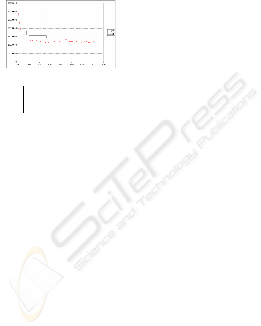
(a) The fitness curves for the correction of the U-
channel.
Y U V
init 49677830 31517024 53538715
SA 23608403 14298870 16127666
ES 20240155 10819027 15581825
(b) The initial and achieved best fitnesses.
Figure 2: Results of the vignetting reduction.
Table 1: Inter-robot calibration. ∆µ
start
, ∆µ
end
represent
the difference of the mode of the robot from the reference
(“alpha”) before and after the calibration. σ
start
, σ
end
are
the standard deviation from the reference mode.
Color ∆µ
start
∆µ
end
σ
start
σ
end
Card Y/U/V Y/U/V Y/U/V Y/U/V
green 1/0/3 1/0/4 6.2/3.8/7.4 3.2/3.0/3.9
orange 18/12/5 7/2/3 13.3/17.8/9.3 4.6/4.8/4.2
cyan 13/2/8 5/2/4 11.3/3.9/4.8 4.4/3.8/4.0
red 4/9/5 2/1/1 7.6/15.2/7.5 3.1/5.2/3.6
yellow 6/7/30 5/4/5 21.5/8.3/24.8 6.0/3.9/5.5
pink 17/6/5 3/1/2 24.6/12.6/8.9 5.3/4.3/5.6
ages much closer to the reference values provided by
the alpha robot. The total optimization time, split in
2 runs (one for the vignetting, the other for the inter-
robot calibration) was approximately 6 minutes.
5 CONCLUSIONS
We have presented a technique to correct chromatic
distortion within an image and to compensate for
color response differences among similar cameras
which equip a team of robots. Since our black-box ap-
proach does not use assumptions concerning the phys-
ical/geometrical roots of the distortion, this approach
can be easily applied to a wide range of camera sen-
sors and can partially deal with some digital sources
of distortion such as clipping / saturation. Its efficient
implementation has a negligible run-time cost, requir-
ing just two look-up operations per pixel, so it is suit-
able for real time applications on resource constrained
platforms.
REFERENCES
Bruce, J., Balch, T., and Veloso, M. (2000). Fast and
inexpensive color image segmentation for interactive
robots. In Proceedings of the 2000 IEEE/RSJ Interna-
tional Conference on Intelligent Robots and Systems
(IROS ’00), volume 3, pages 2061–2066.
Iocchi, L. (2007). Robust color segmentation through adap-
tive color distribution transformation. In RoboCup
2006: Robot Soccer World Cup X, Lecture Notes in
Artificial Intelligence. Springer.
Kang, S. B. and Weiss, R. S. (2000). Can we calibrate a
camera using an image of a flat, textureless lambertian
surface? In ECCV ’00: Proceedings of the 6th Euro-
pean Conference on Computer Vision-Part II, pages
640–653. Springer-Verlag.
Kirkpatrick, S., Gelatt, C. D., and Vecchi, M. P. (1983). Op-
timization by simulated annealing. Science, Number
4598, 13 May 1983, 220, 4598:671–680.
Lam, D. C. K. (2004). Visual object recognition using sony
four-legged robots. Master’s thesis, The University
of New South Wales, School of Computer Science &
Engineering.
Manders, C., Aimone, C., and Mann, S. (2004). Camera
response function recovery from different illumina-
tions of identical subject matter. In IEEE International
Conference on Image Processing 2004.
Nanda, H. and Cutler, R. (2001). Practical calibrations for
a real-time digital omnidirectional camera. Technical
report, CVPR 2001 Technical Sketch.
Nistic
`
o, W. and R
¨
ofer, T. (2006). Improving percept reli-
ability in the sony four-legged league. In RoboCup
2005: Robot Soccer World Cup IX, Lecture Notes in
Artificial Intelligence, pages 545–552. Springer.
R
¨
ofer, T. (2004). Quality of ers-7 camera images.
http://www.informatik.uni-bremen.de/˜roefer/ers7/.
Schulz, D. and Fox, D. (2004). Bayesian color estimation
for adaptive vision-based robot localization. In Pro-
ceedings of IROS.
Schwefel, H.-P. (1995). Evolution and Optimum Seeking.
Sixth-Generation Computer Technology. Wiley Inter-
science, New York.
Sony Corporation (2004). OPEN-R SDK Model Informa-
tion for ERS-7. Sony Corporation.
Welch, G. and Bishop, G. (2003). An introduction to the
kalman filter.
Xu, J. (2004). Low level vision. Master’s thesis, The Uni-
versity of New South Wales, School of Computer Sci-
ence & Engineering.
REAL-TIME INTER- AND INTRA- CAMERA COLOR MODELING AND CALIBRATION FOR RESOURCE
CONSTRAINED ROBOTIC PLATFORMS
383
