Impact of Data Dimensionality Reduction on Neural

Based Classification: Application to Industrial Defects

Matthieu Voiry

1,2

, Kurosh Madani

, Véronique Amarger

and Joël Bernier

Images, Signals, and Intelligent System Laboratory

(LISSI / EA 3956), Paris-XII – Val de Marne University

Senart Institute of Technology, Avenue Pierre Point, Lieusaint, 77127, France

SAGEM REOSC

Avenue de la Tour Maury, Saint Pierre du Perray, 91280, France

Abstract. A major step for high-quality optical surfaces faults diagnosis con-

cerns scratches and digs defects characterisation. This challenging operation is

very important since it is directly linked with the produced optical component’s

quality. To complete optical devices diagnosis, a classification phase is manda-

tory since a number of correctable defects are usually present beside the poten-

tial “abiding” ones. Unfortunately relevant data extracted from raw image dur-

ing defects detection phase are high dimensional. This can have harmful effect

on behaviors of artificial neural networks which are suitable to perform such a

challenging classification. Reducing data dimension to a smaller value can

however decrease problems related to high dimensionality. In this paper we

compare different techniques which permit dimensionality reduction and evalu-

ate their possible impact on classification tasks performances.

1 Introduction

We are involved in fault diagnosis of optical devices in industrial environment. In

fact, classification of detected faults is among chief phases for succeeding in such

diagnosis. Aesthetic flaws, shaped during different manufacturing steps, could pro-

voke harmful effects on optical devices’ functional specificities, as well as on their

optical performances by generating undesirable scatter light, which could seriously

degrade the expected optical features. Taking into account the above-mentioned

points, a reliable diagnosis of these defects in high-quality optical devices becomes a

crucial task to ensure products’ nominal specification and to enhance the production

quality. Moreover, the diagnosis of these defects is strongly motivated by manufac-

turing process correction requirements in order to guarantee mass production (repeti-

tive) quality with the aim of maintaining acceptable production yield.

Unfortunately, detecting and measuring such defects is still a challenging dilemma

in production conditions and the few available automatic control solutions remain

ineffective. That’s why, in most of cases, the diagnosis is performed on the basis of a

human expert based visual inspection of the whole production. However, this usual

Voiry M., Madani K., Amarger V. and Bernier J. (2007).

Impact of Data Dimensionality Reduction on Neural Based Classiﬁcation: Application to Industrial Defects.

In Proceedings of the 3rd International Workshop on Artiﬁcial Neural Networks and Intelligent Information Processing, pages 56-65

DOI: 10.5220/0001635500560065

 SciTePress

solution suffers from several acute restrictions related to human operator’s intrinsic

limitations (reduced sensitivity for very small defects, detection exhaustiveness al-

teration due to attentiveness shrinkage, operator’s tiredness and weariness due to

repetitive nature of fault detection and fault diagnosis tasks).

To overcome these problems we have proposed a detection approach based on

Nomarski’s microscopy issued imaging [1] [2]. This method provides robust detec-

tion and reliable measurement of outward defects, making plausible a fully automatic

inspection of optical products. However, the above-mentioned detection process

should be completed by an automatic classification system in order to discriminate the

“false” defects (correctable defects) from “abiding” (permanent) ones. In fact, be-

cause of industrial environment, a number of correctable defects (like dusts or clean-

ing marks) are usually present beside the potential “abiding” defects. That is why the

association of a faults’ classification system to the aforementioned detection module

is a foremost supply to ensure a reliable diagnosis. In a precedent paper [3], we pro-

posed a method to extract relevant data from raw Nomarski images. In the aim of

effectively classify these descriptors, neural network based techniques seem appropri-

ate because they have shown many attractive features in complex pattern recognition

and classification tasks [4] [5]. But we are dealing with high dimensional data (13 and

more components vectors), therefore behaviour of a number of these algorithms could

be affected. To avoid this problem we are investigating different dimension reduction

techniques for achieving better classification (in terms of performance and processing

time).

This paper is organized as follows: in the next section, motivations for reducing

data dimensionality and also SOM, CCA and CDA, three technique carrying out this

task are introduced. These techniques have been tested using an experimental proto-

col presented in Section 3. The Section 4 deals with experiments results: first a com-

parison of data projection quality and an analysis of their possible impact on classifi-

cation tasks are carried out. Secondly this impact is demonstrated on a classification

task involving Multilayer Perceptron artificial neural network. Finally, the Section 5

will conclude this work and will give a number of perspectives.

2 Data Dimensionality Reduction Techniques

It can be found in literature, lot of examples using various dimension reduction tech-

niques (linear or not) as a preliminary step before more refined processing, among

which, Self Organizing Maps (SOM) [6;7], Curvilinear Component Analysis (CCA)

[8;9] and Curvilinear Distance Analysis (CDA) [10].

2.1 The “curse of dimensionality”

Dealing with high-dimensional data indeed poses problems, known as “curse of di-

mensionality” [9]. First, sample number required to reach a predefined level of preci-

sion in approximation tasks, increases exponentially with dimension. Thus, intui-

tively, the sample number needed to properly learn problem becomes quickly much

too large to be collected by real systems, when dimension of data increases. Moreover

surprising phenomena appear when working in high dimension [11] : for example,

variance of distances between vectors remains fixed while its average increases with

the space dimension, and Gaussian kernel local properties are also lost. These last

points explain that behaviour of a number of artificial neural network algorithms

could be affected while dealing with high-dimensional data. Fortunately, most real-

world problem data are located in a manifold of dimension p much smaller than its

raw dimension. Reducing data dimensionality to this smaller value can therefore

decrease the problems related to high dimension.

2.2 Self-Organizing Maps (SOM)

Self-Organizing Map is a classical method originally proposed by Kohonen [12]. This

algorithm projects multidimensional feature space into a low-dimensional presenta-

tion. Typically a SOM consists of a two dimensional grid of neurons. A vector of

features is associated with each neuron. During the training phase, these vectors are

tuned to represent the training data under constraint of neighbourhood conservation.

Similar data are projected to the same or nearby neurons in the SOM, while different

ones are mapped to neurons located further from each other, resulting in clustered

data. Thus, SOM is an efficient tool for quantizing the data’s space and projecting

this space onto a low-dimensional space, while conserving its topology. SOM is often

used in industrial engineering [13], [14] to characterize high-dimensional data or to

carry out classification tasks. Unfortunately it suffers from major drawbacks: first the

configuration of the topology is static and should be fixed a priori (what is efficient

only for little values of projection subspace dimension), moreover the method defines

only a discrete nonlinear subspace, and finally algorithm is computationally too ex-

pensive to be practically applied for projection space dimension higher than 3.

2.3 Curvilinear Component Analysis (CCA)

The goal of this technique proposed by Demartines [15] is to reproduce the topology

of a n-dimension original space in a new p-dimension space (where p<n) without

fixing any configuration of the topology. To do so, a criterion characterizing the dif-

ferences between original and projected space topologies is processed:

∑∑

≠

−=

iij

ijCCA

dFddE )()(

(1)

Where

d (respectively

d ) is the Euclidean distance between vectors

x and

x of

considered distribution in original space (resp. in projected space), and F is a decreas-

ing function which favors local topology with respect to the global topology. This

energy function is minimized by stochastic gradient descent [16]:

),)()(()(,

xxdtu

txji −−

−

=Δ≠∀

λα

(2)

Where

]1;0[: →ℜ

and

ℜ→ℜ:

are two decreasing functions represent-

ing respectively a learning parameter and a neighborhood factor. CCA provides also a

similar method to project, in continuous way, new points in the original space onto

the projected space, using the knowledge of already projected vectors.

2.4 Curvilinear Distance Analysis (CDA)

Since CCA encounters difficulties with unfolding of very non-linear manifolds, an

evolution called CDA has been proposed [17]. It involves curvilinear distances (in

order to better approximate geodesic distances on the considered manifold) instead of

Euclidean ones. Curvilinear distances are processed in two steps way. First is built a

graph between vectors by considering k-NN,

, or other neighbourhood, weighted by

Euclidean distance between adjacent nodes. Then the curvilinear distance between

two vectors is computed as the minimal distance between these vectors in the graph

using Dijkstra’s algorithm. Finally the original CCA algorithm is applied using proc-

essed curvilinear distances. This algorithm allows dealing with very non-linear mani-

folds and is much more robust against the choices of

and

functions.

3 Experimental Validation Protocol

In order to obtain exploitable data for a classification scheme, we first needed to ex-

tract relevant information of raw Nomarski’s microscopy issued images. We pro-

posed to proceed in two steps [2]: first a detected items’ images extraction phase and

then an appropriated coding of the extracted images. The image associated to a given

detected item is constructed considering a stripe of ten pixels around its pixels. Thus

the obtained image gives an isolated (from other items) representation of the defect

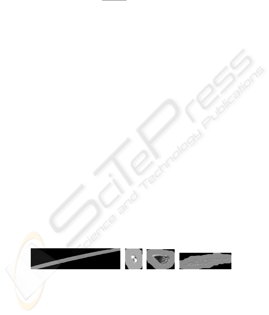
(e.g. depicts the defect in its immediate environment). Figure 1 gives four examples

of detected items’ images using the aforementioned technique. It shows different

characteristic items which could be found on optical device in industrial environment.

b) c) d)

Fig. 1. Images of characteristic items: a) scratch; b) dig; c) dust; d) cleaning marks.

The information contained in such images is highly redundant. Furthermore, the gen-

erated images don’t have necessarily the same dimension (typically this dimension

can turn out to be thousand times as high). That is why these raw data (images) can-

not be directly processed and have to be appropriately encoded. This is done using a

set of Fourier-Mellin transform issued invariants described bellow. The Fourier-

Mellin transform of a function

);(

rf , in polar coordinates, is given by relation (1),

with q∈ Z, s = σ + ip ∈ C (see[18]):

∫∫

∞

−

−=

);()exp();(

ddrrfiqrsqM

θθθ

(3)

In [19], are proposed a set of features invariant on geometric transformation:

[]

[

]

fff

MMMsqMsqI );1();1();0();();(

σσσ

−

(4)

In order to validate the above-presented concepts and to provide an industrial proto-

type, an automatic control system has been realized. It involves an Olympus B52

microscope combined with a Corvus stage, which allows scanning an entire optical

component. 50x magnification is used, that leads to microscopic 1.77mm x 1.33 mm

fields and 1.28µm x 1.28µm sized pixels. These facilities were used to acquire a great

number of defects images. These images were coded using Fourier-Mellin transform

with

and

{}

);1()0;0/(),(),( PpPQqPpqpqpq ≤≤

−

≤

∪

≤

∈

where

and

2=Q

(see Equation 2). Such transform provides a set of 13 features

for each item. Three experiments called A, B, C were carried out, using two optical

devices. Table 1 shows the different parameters corresponding to these experiments.

It’s important to note that, in order to avoid false classes learning, items images de-

picting microscopic field boundaries or two (or more) different defects are discarded

from used database. First, since database C is issued from a cleaned device, it’s con-

stituted with almost only “permanent” defect. And because database B came from the

measurement of the same optical device but without cleaning phase, it’s constituted

with the same type of “permanent” defects but also with “correctable” ones. In the

aim of studying structure of space described by database when reducing its dimen-

sion, we perform some experiments. First a reduction of dimensionality from 13 (raw

dimensionality) to 2 of the database B was performed using SOM, CCA and CDA, in

order to compare projection quality of these three techniques Then the entire data-

base C was projected into the obtained space in order to evaluate the pertinence of

dimensionality reduction for discrimination between “correctable” and “abiding”

defects. Finally a classification task, involving aforementioned databases and Multi-

layer Perceptron artificial neural network, was carried out with and without dimen-

sionality reduction phase with the aim to demonstrate usefulness of such pre-

processing phase.

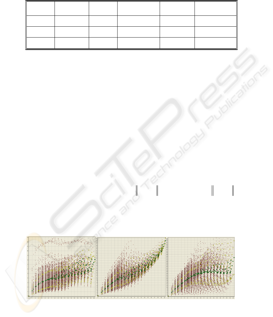
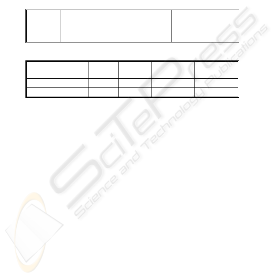
Table 1. Description of the three experiments supplying studied databases.

Database

Optical Device

Identifiant

Cleaning

Number of studied

microscopic fields

Correspondant

studied area

Number of items in

the learning database

A 1 No 1178 28 cm² 3865

B 2 No 605 14 cm² 1910

C 2 Yes 529 12,5 cm² 1544

4 Experimental Results and Analysis

4.1 Quality of Projection

Dimensionality reduction has been performed using the three aforementioned tech-

niques, SOM, ACC and CDA on database B. To compare the results of the three

experiments, the 2-D projections issued from CCA and CDA were processed by a

SOM, using the same shape of grid (20x8) as in the SOM experiment. An important

point is that SOM is just used, in these two last cases, to perform a quantization and

not for dimension reduction, since it works on a 2 dimension space. Therefore, we

can directly compare dimension reduction ability of the different techniques by com-

paring these maps with map obtained by applying SOM’s algorithm on raw data. The

quality evaluation of non-linear projection of the data space onto the neurons grid

space is performed by studying, for each pair of neurons, the dx distance between

these two neurons in the data space, versus the dy distance between these two neurons

in the grid space [20]. For each couple of neurons

);( ji we draw a point

)),();,(( jidxjidy

where

xxjidx

−=),(

and

yyjidy

−=),(

(resp.

) is the vector of features corresponding to the k-th neuron in the data

space (resp. in the grid space). If the topology of the data space is not well respected,

dx is not related to dy and we obtain a diffuse cloud of points. On the contrary, if

neurons organization is correct, the drawn points are almost arranged along a straight

line.

Fig. 2. dy-dx representation of the three obtained SOMs for database B (mean □ and standard

deviation ◊ of dx are also represented). Left: SOM; middle: CCA; right: CDA.

First, in Figure 2, cloud of points is more diffuse for SOM than in the case of CCA,

and the curve constituted by dx averages for each dy less uniformly monotonic. It

reveals the fact that the CCA performs better than SOM, while approximately the

same quantity is minimized. The cloud obtained for CDA is quite different because

dy is related to curvilinear distance and not Euclidean one. The figure is however the

same as for CCA for little dy value, because in these cases Euclidean distance is a

good approximate of curvilinear one (and therefore distribution is locally linear).

4.2 Analysis of Possible Impact on Classification Tasks

We now consider the database C (only “permanent” defects) and project its items

onto the three previously obtained SOMs. We perform also an equivalent experiment

on raw data (13-dimension), using k-means algorithm with k=20x8=160. Since k-

means algorithm has identical behaviour as SOM, except concerning neighbourhood

constraints, it has the same effect on projected items distribution but doesn’t allow

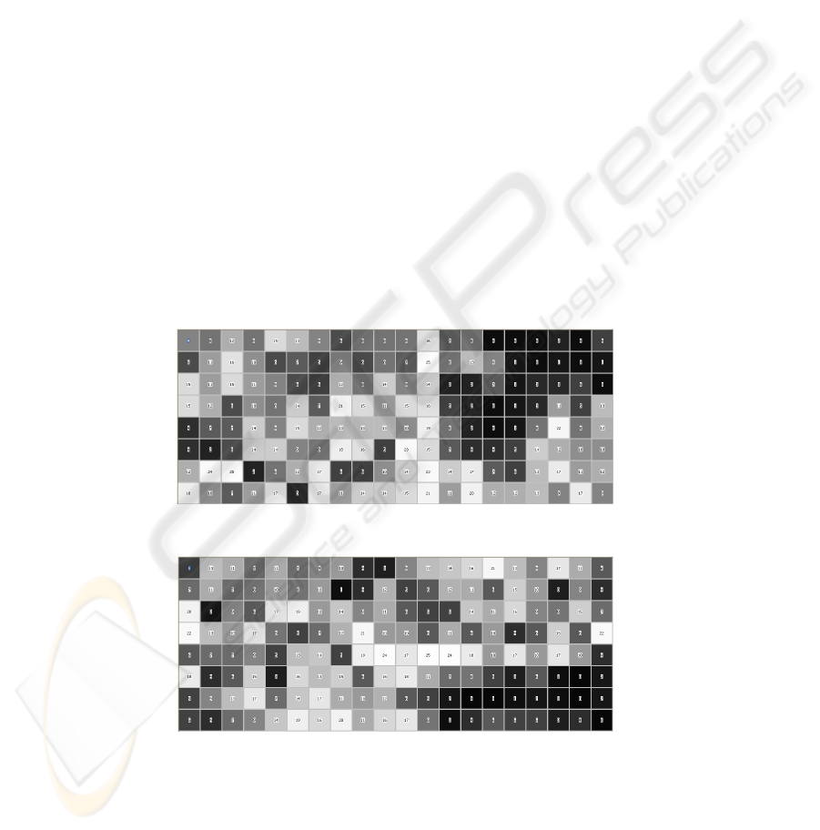
visual representation. Projected items distribution after SOM (Figure 3), CCA (Figure

4) and CDA (Figure 5) dimension reduction are studied. In these figures, the equal-

ized grey level depicts the number of projected items for each SOM’s cell (this num-

ber is also reported in the cell). In table 2 are reported some characteristic values of

permanent defects distributions “homogeneity”: entropy and standard deviation of

projected items number in each cell; number of empty or quasi-empty cells (<3 pro-

jected items).

Fig. 3. Distribution of projected items in SOM map. (SOM reduction dimension).

Fig. 4. Distribution of projected items in SOM map. (CCA reduction dimension).

Maps and numerical measurements for SOM and CCA are comparable and therefore

these techniques are equivalent for the considered problem. CCA is however easier to

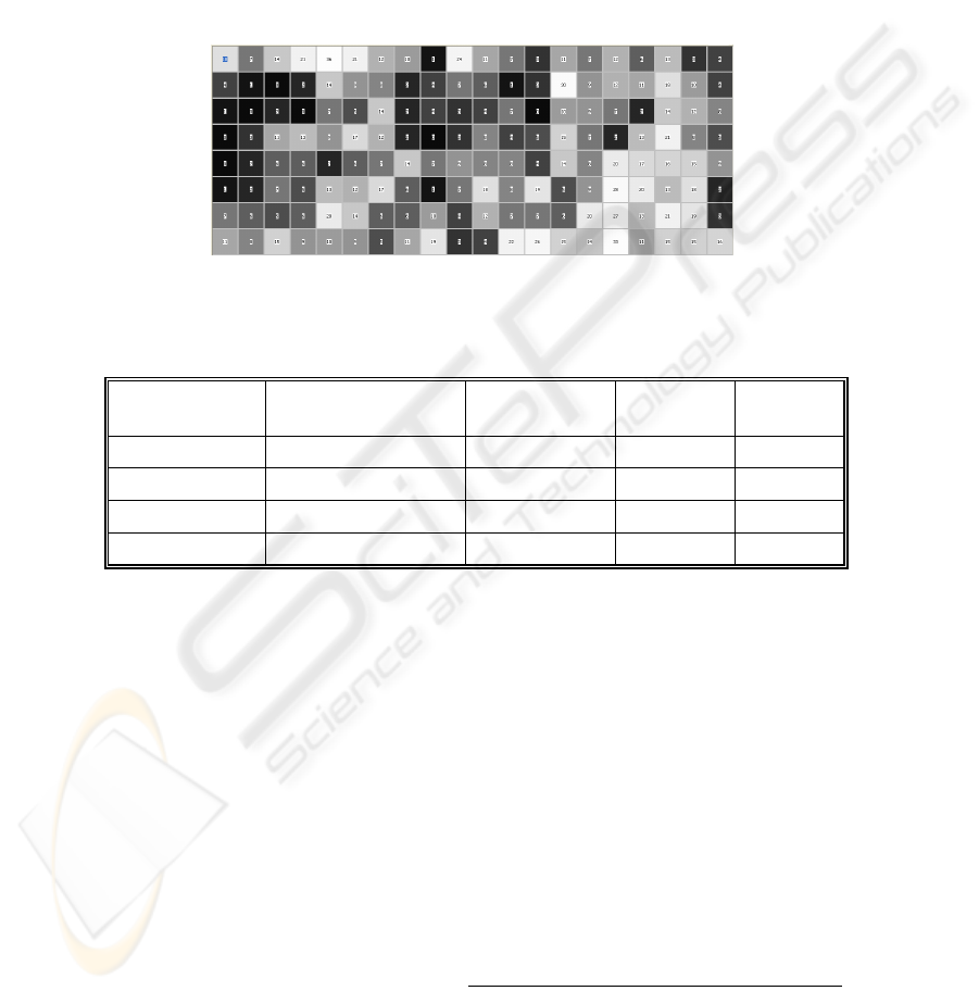
perform (no a priori knowledge or difficult choice) and provide more information

(continuous projection). CDA offers the same advantages as CCA, but it seems to be

more appropriate for pre-processing before classification. Corresponding map depicts

indeed more specific “areas” for database C projected defects. This intuition is con-

firmed by numerical measurements: entropy is lower than in SOM and CCA cases

(better organization), standard deviation is higher (better contrast between full and

empty areas) and there are more quasi-empty cells. We think that this organization is

a foremost guarantee for the dimension reduction to allow a better classification. We

can also remark that results obtained with CDA are fairly similar as those with raw

data; it shows that little information is lost while reducing dimensionality.

Fig. 5. Distribution of projected items in SOM map. (CDA reduction dimension).

Table 2. Different measurements characterizing the projections distribution of database C

items (permanent defects).

Applied dimensional-

ity reduction technique

Standard-deviation of

projected defects distribution

Entropy of projected

defects distribution

Number of

empty cells

Number of

cells with less

than 3 defects

None 8.72 2.055 15 30

SOM 5.78 2.114 9 26

CCA 5.72 2.121 5 20

CDA 7.04 2.088 7 32

4.3 Validation on an Artificial Neural Network Based Classification

We studied a classification problem in order to evaluate pertinence of using dimen-

sion reduction before such task. First, we fixed item labels using obtained SOM with

CDA dimension reduction (see Figure 5). Since database C wasn’t completely consti-

tuted of “permanent” defects (according to an expert, some dusts and cleaning marks

still remain), we chose to label all SOM cells with less than 5 projected items of data-

base C as 1:“probably correctable defects” , and the others as -1:“probably permanent

defects”. Then each item from database A and B was projected into the SOM and

labelled in accordance with its belonging cell, obtaining databases described in Table

3. We performed a first experiment, training a multilayer perceptron with 13 input

neurons, 35 neurons in one hidden layer, and 2 output neurons (13-35-2 MLP)

artificial neural network using BFGS [21] with bayesian regularization algorithm with

database 2. Then a second experiment was carried out, training a 2-25-2 MLP

artificial neural network with database 2 after CDA 2-dimensional space reduction

For these two experiments, training was achieved 20 times and the generalization

ability of obtained neural networks was processed using database 1. Results are

presented in Table 4. Since database 1 and database 2 came from different optical

devices, these generalization results are significant. These results clearly prove that

the considered classification problem can be simplified, when properly reformulated

in a dimension lower than its raw dimensionality and in accord with its real

dimensionality.

Table 3. Description of classification databases.

Database Coming from database Total number of items Label 1 items Label –1 items

1 A 3865 1046 2816

2 B 1910 489 1421

Table 4. MLP classification performances on database 1.

CDA Reduc-

tion Dimen-

sion

Training

database

dimensionality

Class 1 items

Well-

Recognized

Class -1 items

Well-

Recognized

Global

Performance of good

classification

Global Performance

Standard Deviation

No 13 71.6 % 78.0 %

76.27 %

1.,37 %

Yes 2 87.4 % 96.7 %

94.16 %

0.87 %

5 Conclusion and Perspectives

A reliable diagnosis of aesthetic flaws in high-quality optical devices is a crucial task

to ensure products’ nominal specification and to enhance the production quality by

studying the impact of the process on such defects. To ensure a reliable diagnosis, an

automatic classification system is needed in order to discriminate the “correctable”

defects from “abiding” ones. Unfortunately relevant data extracted from raw Nomar-

ski image during defects detection phase are high dimensional. This can have harmful

effect on behaviors of artificial neural networks which are suitable to perform such a

challenging classification. Reducing the dimension of the data to a smaller value can

decrease the problems related to high dimension. In this paper we have compared

different techniques, SOM, CCA and CDA which permit such dimensionality reduc-

tion and evaluated their impact on classification tasks involving real industrial data.

CDA seems to be the most suitable technique and we have demonstrated its ability to

enhance performances in a synthetic classification task. Next phase of this work will

deal with a classification task on data previously labeled by an expert.

References

1. M. Voiry, F. Houbre, V. Amarger, and K. Madani: Toward Surface Imperfections Diagno-

sis Using Optical Microscopy Imaging in Industrial Environment.IAR & ACD, p.139-144

(2005).

2. M. Voiry, V. Amarger, K. Madani, and F. Houbre: Combining Image Processing and Self

Organizing Artificial Neural Network Based Approaches for Industrial Process Faults Clus-

tering . 13th International Multi-Conference on Advanced Computer Systems, p.129-138

(2006).

3. M. Voiry, K. Madani, V. Amarger, and F. Houbre: Toward Automatic Defects Clustering

in Industrial Production Process Combining Optical Detection and Unsupervised Artificial

Neural Network Techniques. Procedings of the 2nd International Workshop on Artificial

Neural Networks and Intelligent Information Processing - ANNIIP 2006, p.25-34 (2006).

4. G. P. Zhang: Neural Networks for Classification: A Survey, IEEE Trans. on Systems, Man,

and Cybernetics - Part C: Applications and Reviews, vol. 30, no. 4, p.451-462 (2000).

5. M. Egmont-Petersen, D. de Ridder, and H. Handels : Image Processing with Neural Net-

works - A Review, Pattern Recognition, vol. 35, p.2279-2301 (2002).

6. K. Boehm, W. Broll, and M. Sokolewicz: Dynamic Gesture Recognition Using Neural

Networks; A Fundament for Advanced Interaction Construction, Proceedings of SPIE, vol.

2177, Stereoscopic Displays and Virtual Reality Systems (1994).

7. J. Lampinen and E. Oja: Distortion Tolerant Pattern Recognition Based on Self-Organizing

Feature Extraction, IEEE Trans. on Neural Networks vol. 6, p.539-547(1995).

8. S. Buchala, N. Davey, T. M. Gale, and R. J. Frank: Analysis of Linear and Nonlinear

Dimensionality Reduction Methods for Gender Classifcation of Face Images, International

Journal of Systems Science (2005).

9. M. Verleysen: Learning high-dimensional data. LFTNC'2001 - NATO Advanced Research

Workshop on Limitations and Future Trends in Neural Computing (2001).

10. M. Lennon, G. Mercier, M. C. Mouchot, and L. Hubert-Moy: Curvilinear Component

Analysis for Nonlinear Dimensionality Reduction of Hyperspectral Images, Proceedings of

SPIE, vol. 4541, Image and Signal Processing for Remote Sensing VII, p.157-168 (2001).

11. P. Demartines, "Analyse de Données par Réseaux de Neurones Auto-Organisés." PhD

Thesis, Institut National Polytechnique de Grenoble (1994).

12. T. Kohonen: Self Organizing Maps, 3rd edition ed. Berlin: Springer (2001).

13. T. Kohonen, E. Oja, O. Simula, A. Visa, and J. Kangas: Engineering Applications of the

Self-Organizing Maps, Proceedings of the IEEE, vol. 84, no. 10, p.1358-1384 (1996).

14. J. Heikkonen and J. Lampinen: Building Industrial Applications with Neural Net-

works.,Proc.European Symposium on Intelligent Techniques, ESIT'99 (1999).

15. P. Demartines and J. Hérault: Vector Quantization and Projection Neural Network, Lecture

Notes in Computer Science, vol. 686, International Workshop on Artificial Neural Net-

works, p.328-333 (1993).

16. P. Demartines and J. Hérault: CCA : "Curvilinear Component Analysis", Proceedings of

15th workshop GRETSI (1995).

17. J. A. Lee, A. Lendasse, N. Donckers, and M. Verleysen: A Robust Nonlinear Projection

Method, European Symposium on Artificial Neural Networks - ESANN'2000 (2000).

18. S. Derrode, "Représentation de Formes Planes à Niveaux de Gris par Différentes Approxi-

mations de Fourier-Mellin Analytique en vue d'Indexation de Bases d'Images." PhD Thesis

, Université de Rennes I (1999).

19. F. Ghorbel: A Complete Invariant Description for Gray Level Images by the Harmonic

Analysis Approach, Pattern Recognition, vol. 15, p.1043-1051 (1994).

20. P. Demartines and F. Blayo: Kohonen Self-Organizing Maps:Is the Normalization Neces-

sary?, Complex Systems, vol. 6, no. 2, p.105-123 (1992).

21. J. E. Dennis and R. B. Schnabel: Numerical Methods for Unconstrained Optimization and

Nonlinear Equations. Englewood Cliffs, NJ: Prentice Hall (1983).