PREDICTIVE CONTROL BY LOCAL VISUAL DATA

Mobile Robot Model Predictive Control Strategies Using Local Visual

Information and Odometer Data

Lluis Pacheco and Ningsu Luo

Institute of Informatics and Applications, University of Girona, Av. Ll. Santaló s/n, Girona, Spain

Keywords: Autonomous mobile robots, computer vision control, system identification, model based control, predictive

control, trajectory planning, obstacle avoidance, robot vision.

Abstract: Nowadays, the local visual perception research, applied to autonomous mobile robots, has succeeded in

some important objectives, such as feasible obstacle detection and structure knowledge. This work relates

the on-robot visual perception and odometer system information with the nonlinear mobile robot control

system, consisting in a differential driven robot with a free rotating wheel. The description of the proposed

algorithms can be considered as an interesting aspect of this report. It is developed an easily portable

methodology to plan the goal achievement by using the visual data as an available source of positions.

Moreover, the dynamic interactions of the robotic system arise from the knowledge of a set of experimental

robot models that allow the development of model predictive control strategies based on the mobile robot

platform PRIM available in the Laboratory of Robotics and Computer Vision. The meaningful contribution

is the use of the local visual information as an occupancy grid where a local trajectory approaches the robot

to the final desired configuration, while avoiding obstacle collisions. Hence, the research is focused on the

experimental aspects. Finally, conclusions on the overall work are drawn.

1 INTRODUCTION

The research presented in this paper addresses to a

kind of differential driven WMRs (wheeled mobile

robots). Nowadays, the computer vision techniques

applied to WMR have solved the problem of

obstacle detection by using different methods as

stereo vision systems, optical flow or DFF (depth

from focus). Stereo vision systems seem to provide

the easiest cues to infer scene depth (Horn, 1998).

The optical flow techniques used in WMR result in

several applications as i.e. structure knowledge,

obstacle avoidance, or visual servoing (Campbell, et

al., 2004). The DFF methods are also suitable for

WMR. For example, three different focused images

were used, with almost the same scene, acquired

with three different cameras

(Nourbakhsh, et al.,

1997). In this work, it is supposed that available

obstacle positions are provided by using computer

vision systems. In this context, the allowed

navigation control signals should achieve the

obstacle avoidance as well as the final desired

coordinates. Scientific community has developed

several studies in this field. Based on the dynamic

window approach with available robot speeds, the

reactive avoidance collisions, safety stop and goal

can be achieved using the dynamic constraints of

WMR (Fox, et al., 1997).

Rimon and Koditschek

(1992) presented the methodologies for the exact

motion planning and control, based on the artificial

potential fields where the complete information

about the free space and goal are encoded. Some

approaches on mobile robots propose the use of

potential fields, which satisfy the stability in a

Lyapunov sense, in a short prediction horizon

(Ögren and Leonard, 2005). The main contribution

of this paper is the use of the visual information as a

dynamic window where the collision avoidance and

safety stop can be planned. Thus, local visual data,

instead of artificial potential fields, are used in order

to achieve the Lyapunov stability. The use of MPC

(model predictive control) with available on-robot

information is possible. Moreover, the local visual

information is used as an occupancy grid that allows

planning feasible trajectories towards the desired

objective. The knowledge of the objective allows the

optimal solution of the local desired coordinates

based on the acquired images. The sensor fusion is

done using visual perception, as the meaningful

source of information in order to accomplish with

the robot tasks. Other data provided by the encoder-

based odometer system are also considered.

259

Pacheco L. and Luo N. (2007).

PREDICTIVE CONTROL BY LOCAL VISUAL DATA - Mobile Robot Model Predictive Control Strategies Using Local Visual Information and Odometer

Data.

In Proceedings of the Fourth International Conference on Informatics in Control, Automation and Robotics, pages 259-266

DOI: 10.5220/0001638102590266

 SciTePress

This paper is organized as follows: Section 1

gives a brief presentation about the aim of the

present work. In the Section 2, the platform is

introduced as an electromechanical system. This

section also describes the experiments to be realized

in order to find the parametric model of the robot

suitable for designing and implementing MPC

methods. In the Section 3, the use of visual data is

presented as a horizon where optimal trajectories can

be planned. Section 4 presents the MPC strategies

used for achieving the path following of the

reference trajectories. In the Section 5, some

conclusions are made with special attention paid into

the future research works.

2 ROBOT AND BASIC CONTROL

METHODS

This section gives some description on the main

robot electromechanical and sensorial systems of the

platform tested in this work. Hence, the WMR

PRIM, available in our lab, has been used in order to

test and orient the research. The experimental

modelling methodologies as well as the model

predictive control are also introduced.

2.1 Electromechanical and Sensorial

System of the Robot

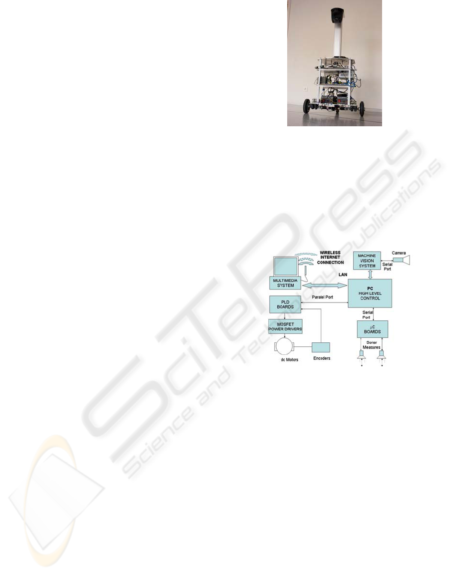
Figure 1 shows the robot PRIM used in the research

work. The mechanical structure of the robot is made

of aluminum, with two independent wheels of 16cm

diameters actuated by two DC motors. The distance

between two wheels is 56.4cm. A third spherical

omni-directional wheel is used to guarantee the

system stability. The maximum continuous torque of

each motor is 131mNm. The proportion of gear

reduction for each motor is 86:1 and thus the total

force actuating on the robot is near 141N. Shaft

encoders with 500 counts/rev are placed at the motor

axes, which provide 43000 counts for each turn of

the wheel. A set of PLD (programmable logic

device) boards is connected to the digital outputs of

the shaft encoders. The printed circuits boards

(PCB) are used to measure the speed of each motor

at every 25ms.

An absolute counter provides the counts in

order to measure the robot position by the odometer

system. Another objective of these boards is to

generate a signal of 23khz PWM for each motor.

The communication between the central digital

can computer and the boards is made through the

thus it parallel port. The speed is commanded by a

byte and generate from 0 to 127 advancing or rever-

Figure 1: The robot PRIM used in this work.

sing speed commands. The maximal speed is near

0.5m/s. A set of microcontroller boards (MCS-51) is

used to read the information available from different

connected sensors. The rate of communication with

these boards is 9600 b/s. Figure 2 shows the

electronic and sensorial system blocks. The data

gathering and the control by digital computer is set

to 100ms.

Figure 2: The sensorial and electronic system blocs.

The system flexibility is increased with the

possibility of connecting with other computer

systems through a local LAN. In this research, it is

connected to a machine vision system that controls a

colour camera EVI-D70P-PAL through the VISCA

RS232-C control protocol. For instance, the camera

configuration used in this work is of a horizontal

field of view of 48º, and a vertical field of 37º. The

focus, pan and tilt remain fixed under present

configuration. Hence, the camera pose is set to

109cm from the floor with a tilt angle of 32º. The

local desired coordinates, obtained by the visual

perception information, are transmitted to the control

unit connecting the USB port to the LAN.

2.2 Experimental Model

The parametric identification process is based on

black box models (Lju, 1989), (Norton, 1986) and

(Van Overschee, Moor, 1996). Thus, the transfer

functions are related to a set of polynomials that

ICINCO 2007 - International Conference on Informatics in Control, Automation and Robotics

260

allow the use of analytic methods in order to deal

with the problem of controller design. The

nonholonomic system dealt with in this work is

considered initially as a MIMO (multiple input

multiple output) system, which is composed of a set

of SISO subsystems with coupled dynamic influence

between two DC motors. The approach of multiple

transfer functions consists in making the

experiments with different speeds. In order to find a

reduced-order model, several studies and

experiments have been done through the system

identification and model simplification.

2.2.1 System Identification

The parameter estimation is done by using a PRBS

(Pseudo Random Binary Signal) as excitation input

signal. It guarantees the correct excitation of all

dynamic sensible modes of the system along the

spectral range and thus results in an accurate

precision of parameter estimation. The experiments

to be realized consist in exciting two DC motors in

different (low, medium and high) ranges of speed.

The ARX (auto-regressive with external input)

structure has been used to identify the parameters of

the robot system. The problem consists in finding a

model that minimizes the error between the real and

estimated data. By expressing the ARX equation as a

lineal regression, the estimated output can be written

as:

θϕ

(1)

with being the estimated output vector, θ the

vector of estimated parameters and φ the vector of

measured input and output variables. By using the

coupled system structure, the transfer function of the

robot can be expressed as follows:

where Y

and Y

represent the speeds of right and

left wheels, and U

and U

the corresponding speed

commands, respectively. In order to know the

dynamics of robot system, the matrix of transfer

function should be identified. Figure 3 shows the

speed response of the left wheel corresponding to a

left PBRS input signal.

Figure 3: Left speed output for a left PRBS input signal.

The treatment of experimental data is done

before the parameter estimation. In concrete, it

includes the data filtering, using the average value of

five different experiments with the same input

signal, the frequency filtering and the tendency

suppression. The system is identified by using the

identification toolbox “ident” of Matlab for second

order models. The following continuous transfer

function matrix for medium speed is obtained:

(3)

⎟

⎠

⎞

⎜

⎝

⎛

⎟

⎠

⎞

⎜

⎝

⎛

⎟

⎠

⎞

⎜

⎝

⎛

89.484.5

12.572.111.0

89.484.5

28.041.326.0

89.484.5

32.027.002.0

89.484.5

46.482.435.0

It is shown by simulation results that the obtained

model fits well with the experimental data.

2.2.2 Simplified Model of the System

This section studies the coupling effects and the way

for obtaining a reduced-order dynamic model. It is

seen from (3) that the dynamics of two DC motors

are different and the steady gains of coupling terms

are relatively small (less than 20% of the gains of

main diagonal terms). Thus, it is reasonable to

neglect the coupling dynamics so as to obtain a

simplified model.

(2)

RRRLRR

LRLLLL

YGGU

⎛⎞⎛ ⎞⎛ ⎞

⎜⎟⎜ ⎟⎜ ⎟

⎝⎠⎝ ⎠⎝ ⎠

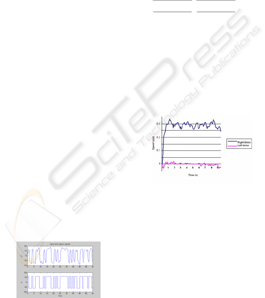
Figure 4: Coupling effects at the left wheel.

In order to verify it from real results, a set of

experiments have been done by sending a zero speed

command to one motor and other non-zero speed

commands to the other motor. In Figure 4, it is

shown a response obtained on the left wheel, when a

medium speed command is sent to the right wheel.

The experimental result confirms the above facts.

The existence of different gains in steady state is

also verified experimentally. Finally, the order

reduction of system model is carried out trough the

analysis of pole positions by using the method of

root locus. Afterwards, the system models are

validated through the experimental data by using the

PBRS input signal. A two dimensional array with

three different models for each wheel is obtained.

Hence, each model has an interval of validity where

the transfer function is considered as linear.

PREDICTIVE CONTROL BY LOCAL VISUAL DATA - Mobile Robot Model Predictive Control Strategies Using Local

Visual Information and Odometer Data

261

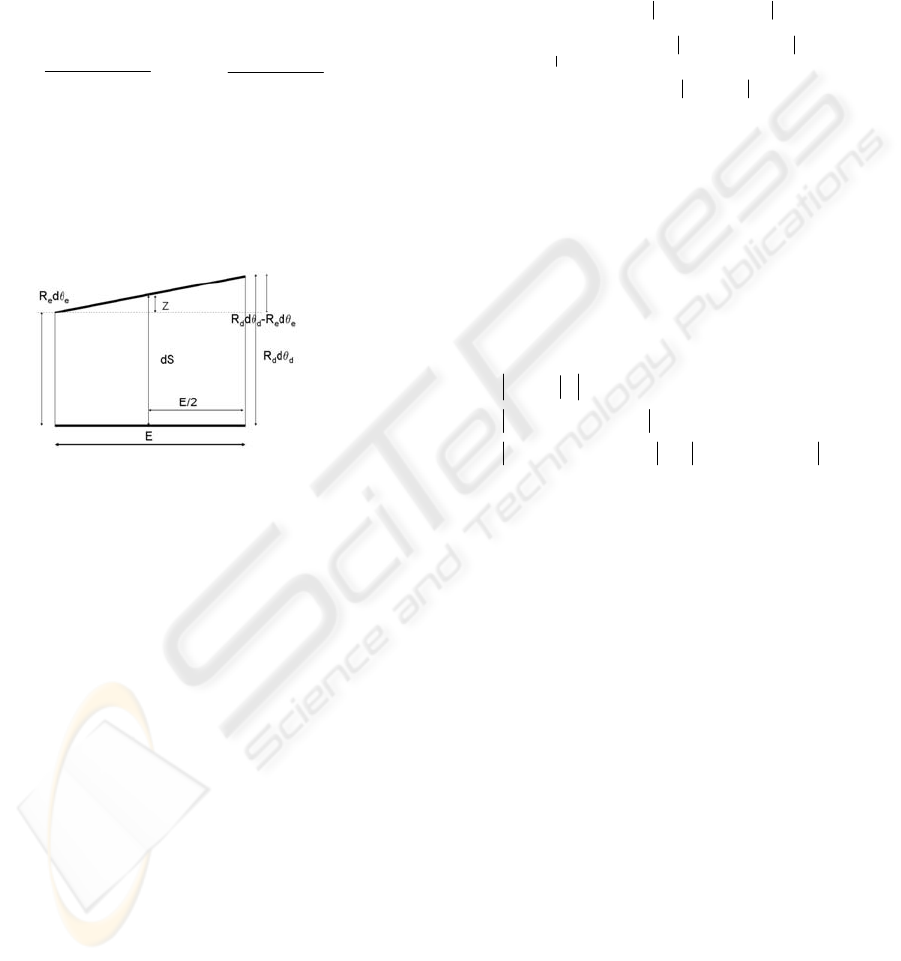
2.3 Odometer System Expression

Denote (x, y, θ) as the coordinates of position and

orientation, respectively. The Figure 5 describes the

positioning of robot as a function of the radius of left

and right wheels (R

, R

), and the angular

incremental positioning (θ

, θ

), with E being the

distance between two wheels and dS the incremental

displacement of the robot. The position and angular

incremental displacements are expressed as:

The coordinates (x, y, θ) can be expressed as:

Figure 5: Positioning of the robot as functions of the

angular movement of each wheel.

Thus, the incremental position of the robot can be

obtained through the odometer system with the

available encoder information obtained from (4) and

(5).

2.4 Model Predictive Control

The model predictive control, MPC, has many

interesting aspects for its application to mobile robot

control. It is the most effective advanced control

technique, as compared to the standard PID control,

that has made a significant impact to the industrial

process control (Maciejowski, 2002). Recently, real

time mobile robot MPC implementations have been

developed using global vision sensing (Gupta,

Messom et al., 2005). In (Küne, Lages et al., 2005),

it was studied the MPC based optimal control useful

for the case when nonlinear mobile robots are used

under several constraints, as well as the real time

implementation possibilities when short prediction

horizons are used. In general, the global trajectory

planning becomes unfeasible since the sensorial

system of some robots is just local. By using a MPC,

the idea of the receding horizon can deal with the

local sensor information. In this way, it is proposed a

local model predictive control, LMPC, in order to

use the available visual data in the navigation

strategies for the goal achievement.

The MPC is based on minimizing a cost

function, related to the objectives, through the

selection of the optimal inputs. In this case, the cost

function can be expressed as follows:

Denote X

=(x

) as the desired coordinates. The

first term of (6) is referred to the final desired

coordinate achievement, the second term to the

trajectory to be followed, and the last one to the

input signals minimization. The parameters P, Q and

R are weighting parameters. X(k+n|k) represents the

terminal value of the predicted output after the

horizon of prediction n and X(k+i|k) represents the

predicted output values within the prediction

horizon. The system constrains are also considered:

The limitation of the input signal is taken into

account in the first constraint. The second constraint

is related to the obstacle points where the robot

should avoid the collision. The last one is just a

convergence criterion.

3 THE HORIZON OF LOCAL

VISUAL PERCEPTION

The use of sensor information as a useful source to

build 2D environment models consists of a free or

occupied grid proposed by (Elfes, 1989). The

knowledge of occupancy grids knowledge has been

used for static indoor mapping with a 2D grid

(Thrun, 2002). In other works of multidimensional

grids, multi target tracking algorithms are employed

by using obstacle state space with Bayesian filtering

techniques (Coué et al., 2006). In this work it is

proposed the use of the local visual information

available from the camera as a local map that has

enough information in order to achieve a global

objective. The occupancy grid can be obtained in

real time by using computer vision methods. The use

of the optical flow has been proposed as a feasible

eedd

dRdR

()

dRdR

eedd

−

()

[]

()

[]

()

[]

()

[]

()()

(6) min,

⎪

⎭

⎪

⎬

⎫

⎪

⎩

⎪

⎨

⎧

+++

−+−++

−+−+

∑

−

⎭

⎬

⎫

⎩

⎨

⎧

−=

kikRUkikU

XkikXQXkikX

XknkXPXknkX

mnJ

kikU

(

)

[][]

[][][][]

()

,,,,

)1,0[

⎪

⎭

⎪

⎬

⎫

⎪

⎩

⎪

⎨

⎧

−≤−

≥−

∈≤+

ddkkddnknk

ooikik

yxyxyxyx

Gyxyx

GkikU

()

θθθ

θθ

ddSyy

ddSxx

nnn

++=

−

−−

5sin

cos

ICINCO 2007 - International Conference on Informatics in Control, Automation and Robotics

262

obstacle avoidance method; as i.e., (Campbell et al.,

2004), in which it was used a Canny edge detector

algorithm that consists in Gaussian filtering and

edge detection by using Sobel filters. Thus, optical

flow was computed over the edges providing

obstacle structure knowledge. The present work

assumes that the occupancy grid is obtained by the

machine vision system. It is proposed an algorithm

that computes the local optimal desired coordinate as

well as the local trajectory to be reached. The

research developed assumes indoor environments as

well as flat floor constraints. However, it can be also

applied in outdoor environments.

This section presents firstly the local map

relationships with the camera configuration and

poses. Hence, the scene perception coordinates are

computed. Then, the optimal control navigation

strategy is presented, which uses the available visual

data as a horizon of perception. From each frame, it

is computed the optimal local coordinates that

should be reached in order to achieve the desired

objective. Finally, the algorithm dealing with the

visual data process is explained. Some involved

considerations are also made.

3.1 Scene Perception

The local visual data provided by the camera are

used in order to plan a feasible trajectory and to

avoid the obstacle collision. The scene available

coordinates appear as an image, where each pixel

coordinates correspond to a 3D scene coordinates. In

the case attaining to this work, flat floor surface is

assumed. Hence, scene coordinates can be computed

using camera setup and pose knowledge, and

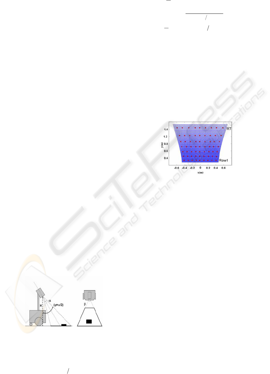
assuming projective perspective. The Figure 6 shows

the robot configuration studied in this work. The

angles

and

are related to the vertical and

horizontal field of view, and the tilt camera pose,

respectively. The vertical coordinate of the camera is

represented by H.

Figure 6: Fixed camera configuration including vertical

and horizontal field of view, and vertical tilt angle.

Using trigonometric relationships, the scene

coordinates can be computed:

(

)

(8)

Δ+

−

= 2tanHy

(

)

≤≤=Δ

()

(9)

ααϕ

Δ+−

±= tan

2cos

()

≤≤=Δ

The K

and K

are parameters used to cover the

image pixel discrete space. Thus, R and C represent

the image resolution through the total number of

rows and columns. It should be noted that for each

row position, which corresponds to scene

coordinates y

, there exist C column coordinates x

i,j

The above equations provide the available local map

coordinates when no obstacle is detected. Thus,

considering the experimental setup reported in

Section 2, the local on-robot map depicted in Figure

7 is obtained.

Figure 7: Local visual perception free of obstacles, under

x72 or 9x7 low resolution grids.

3.2 Local Optimal Trajectory

The available information provided by the camera is

considered as a local horizon where the trajectory is

planned. Hence, a local map with free obstacle

coordinates is provided. In this sense, the available

local coordinates are shown in Figure 7. It is noted

that low resolution scene grids are used in order to

speed up the computing process.

The minimization of a cost function, which

consists in the Euclidean distance between the

desired coordinates and the available local scene

coordinates, can be optimally solved by finding the

local desired coordinates. Hence, the algorithm

explores the image pixels, IMAGE(i,j), considering

just the free obstacle positions. Once the local

desired point is obtained, a trajectory between the

robot coordinates, at the instant when the frame was

acquired, and the optimal scene coordinates is

planned. Thus, the current robot coordinates are

related to this trajectory, as well as to control

methods.

PREDICTIVE CONTROL BY LOCAL VISUAL DATA - Mobile Robot Model Predictive Control Strategies Using Local

Visual Information and Odometer Data

263

3.3 Algorithms and Constraints

In this subsection, some constraints that arise from

the experimental setup are considered. The narrow

field of view and the fixed camera configuration

make necessary that the robot stays oriented towards

the desired coordinates. WMR movements are

planned based on the local visual data, and always in

advancing sense. Hence, the algorithms provide

local desired coordinates to the control unit. If WMR

orientation is not appropriate, the robot could turn

around itself until a proper orientation is found.

Another possibility is to change the orientation in

advancing sense by the use of the trajectory/robot

orientation difference as the cost function computed

over the available visual data. This subsection

proposes the local optimal suggested algorithms that

have as special features an easy and fast

computation. Some methods are presented in order

to overcome the drawback of local minimal failures.

3.3.1 The Proposed Algorithms

The proposed algorithm, concerning to obtaining the

local visual desired coordinates, consists of two

simple steps:

 To obtain the column corresponding to best

optimal coordinates that will be the local desired

coordinate.

 To obtain the closer obstacle row, which will be

the local desired Y

coordinate.

The proposed algorithm can be considered as a first

order approach, using a gross motion planning over

a low resolution grid. The obstacle coordinates are

increased in size with the path width of the robot

(Schilling, 1990). Consequently, the range of

visually available orientations is reduced by the path

width of WMR. Other important aspects as visual

dead zone, dynamic reactive distance and safety stop

distance should be considered. The dynamic reactive

distance, which should be bigger than the visual

dead zone and safety stop distance, is related to the

robot dynamics and the processing time for each

frame. Moreover, the trajectory situated in the visual

map should be larger than a dynamic reactive

distance. Thus, by using the models corresponding

to the WMR PRIM, three different dynamic reactive

distances are found. As i.e. considering a vision

system that processes 4 frames each second, using a

model of medium speed (0.3m/s) with safety stop

distance of 0.25m and an environment where the

velocity of mobile objects is less than 0.5m/s, a

dynamic reactive distance of 0.45m is obtained.

Hence, the allowed visual trajectory distance will set

the speed that can be reached. The desired local

coordinates are considered as final points, until not

any new optimal local desired coordinates are

provided. The image information is explored starting

at the closer positions, from bottom to upside. It is

suggested to speed up the computing process based

on a previously calculated LUT, (look up table),

with the scene floor coordinates corresponding to

each pixel.

3.3.2 Local Minimal Failures

The local minimal failures will be produced when a

convergence criterion, similar to that used in (7), is

not satisfied. Thus, the local visual map cannot

provide with closer optimal desired coordinates,

because obstacles blocks the trajectory to the goal.

In these situations, obstacle contour tracking is

proposed. Hence, local objectives for contour

tracking are used, instead of the goal coordinates, as

the source for obtaining a path until the feasible goal

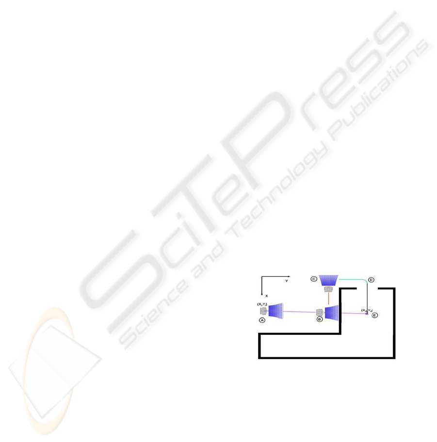
trajectories are found. The Figure 8 shows an

example with local minimal failures. It is seen that

in A, the optimal trajectory is a straight line between

A and E. However, an obstacle is met at B, and local

minimal failure is produced at B. When this is

produced, no trajectory can approach to the desired

goal, (Xd, Yd). Then, obstacle con-tour tracking is

proposed between B and C. Once C is attained, local

minimization along coordinates Y is found and the

trajectory between C and D is planned. From D to E

local minimums are reached until the final goal is

achieved. It should be noted that once B is reached,

the left or right obstacle contour are possible.

However, the right direction will bring the robot to

an increasing Y

distance.

Figure 8: Example of local minimal failures produced at B

with A being the starting point and E the desired goal.

The robot follows the desired goals except when the

situation of obstacle contour tracking is produced,

and then local objectives are just the contour

following points. The local minimal failures can be

considered as a drawback that should be overcome

with more efforts. In this sense, the vision

navigation strategies (Desouza, Kak, 2002) should

be considered. Hence, it is proposed the use of

feasible maps or landmarks in order to provide local

ICINCO 2007 - International Conference on Informatics in Control, Automation and Robotics

264

objective coordinates that can be used for guiding

the WMR to reach the final goal coordinates.

4 LMPC ALGORITHMS

This section gives the LMPC algorithms by using

the basic ideas presented in the Section 2. The

LMPC algorithm is run in the following steps:

 To read the actual position

 To minimize the cost function and to obtain a

series of optimal input signals

 To choose the first obtained input signal as the

command signal.

 To go back to the step 1 in the next sampling

period

The minimization of the cost function is a

nonlinear problem in which the following equation

should be verified:

()()()

(

)

10 yfxfyxf

+≤+

It is a convex optimization problem caused by the

trigonometric functions used in (5), (Boyd,

Vandenberghe, 2004). The use of interior point

methods can solve the above problem (Nesterov,

Nemirovskii, 1994). Among many algorithms that

can solve the optimization, the descent methods are

used, such as the gradient descent method among

others, (Dennis, et al. 1996), (Ortega, et al. 2000).

The gradient descent algorithm has been

implemented in this work. In order to obtain the

optimal solution, some constraints over the inputs

are taken into account:

 The signal increment is kept fixed within the

prediction horizon.

 The input signals remain constant during the

remaining interval of time

The input constraints present advantages such like

the reduction in the computation time and the

smooth behavior of the robot during the prediction

horizon. Thus, the set of available input is reduced to

one value. In order to reduce the optimal signal

value search, the possible input sets are considered

as a bidimensional array, as shown in Figure 9.

Figure 9: Optimal interval search.

Then, the array is decomposed into four zones, and

the search is just located to analyze the center points

of each zone. It is considered the region that offers

better optimization, where the algorithm is repeated

for each sub-zone, until no sub-interval can be

found. Once the algorithm is proposed, several

simulations have been carried out in order to verify

the effectiveness, and then to make the

improvements. Thus, when only the desired

coordinates are considered, the robot could not

arrive in the final point. Figure 10 shows that the

inputs can minimize the cost function by shifting the

robot position to the left.

Figure 10: The left deviation is due to the greater left gain

of the robot.

The reason can be found in (3), where the left motor

has more gain than the right. This problem can be

easily solved by considering a straight-line trajectory

from the actual point of the robot to the final desired

point. Thus, the trajectory should be included into

the LMPC cost function. The Figure 11 shows a

simulated result of LMPC for WMR obtained by

using firstly the orientation error as cost function

and then the local trajectory distance and the final

desired point for the optimization. The prediction

horizons between 0.5s and 1s were proposed and the

computation time for each LMPC step was set to

less than 100ms, running in an embedded PC of

700MHz. In the present research, the available

horizon is provided by using the information of local

visual data. Thus, the desired local points as well as

the optimal local trajectory are computed using

machine vision information.

Figure 11: LMPC simulated results with a 45º trajectory.

5 CONCLUSIONS

This paper has integrated the control science and the

robot vision knowledge into a computer science

environment. Hence, global path planning by using

PREDICTIVE CONTROL BY LOCAL VISUAL DATA - Mobile Robot Model Predictive Control Strategies Using Local

Visual Information and Odometer Data

265

local information is reported. One of the important

aspects of the paper has been the simplicity, as well

as the easy and direct applicability of the

approaches. The proposed methodology has been

attained by using the on-robot local visual

information, acquired by a camera, and the

techniques of LMPC. The use of sensor fusion,

specially the odometer system information, is of a

great importance. The odometer system uses are not

just constrained to the control of the velocity of each

wheel. Thus, the absolute robot coordinates have

been used for planning a trajectory to the desired

global or local objectives. The local trajectory

planning has been done using the relative robot

coordinates, corresponding to the instant when the

frame was acquired. The available local visual data

provides a local map, where the feasible local

minimal goal is selected, considering obstacle

avoidance politics.

Nowadays, the research is focused to implement the

presented methods through developing flexible

software tools that should allow to test the vision

methods and to create locally readable virtual

obstacle maps. The use of virtual visual information

can be useful for testing the robot under synthetic

environments and simulating different camera

configurations. The MPC studies analyzing the

models derived from experiments as well as the

relative performance with respect to other control

laws should also be developed.

ACKNOWLEDGEMENTS

This work has been partially funded the Commission

of Science and Technology of Spain (CICYT)

through the coordinated research projects DPI-2005-

08668-C03, CTM-2004-04205-MAR and by the

government of Catalonia through SGR00296.

REFERENCES

Boyd, S., Vandenberghe, L., 2004. Convex Optimization,

Cambridge University Press.

Campbell, J., Sukthankar, R., Nourbakhsh, I., 2004.

Techniques for Evaluating Optical Flow in Extreme

Terrain, IROS.

Coué, C., Pradalier, C., Laugier, C., Fraichard, T.,

Bessière, P., 2006. Bayesian Occupancy Filtering for

Multitarget Tracking: An Automotive Application,

International Journal of Robotics Research.

Dennis, J.E., Shnabel, R.S., 1996. Numerical Methods for

Unconstrained Optimization and Nonlinear Equations,

Society for Industrial and Applied Mathematics.

DeSouza, G.N., Kak, A.C., 2002. Vision for Mobile Robot

Navigation: a survey, PAMI, 24, 237-267.

Elfes, A., 1989. Using occupancy grids for mobile robot

perception and navigation, IEEE Computer, 22, 46-

57.

Fox, D., Burgard, W., and Thun, S., 1997. The dynamic

window approach to collision avoidance, IEEE Robot.

Autom. Mag. 4, 23-33.

Gupta, G.S., Messom, C.H., Demidenko, S., 2005. Real-

time identification and predictive control of fast

mobile robots using global vision sensor, IEEE Trans.

On Instr. and Measurement, 54, 1.

Horn, B. K. P., 1998. Robot Vision, Ed. McGraw –Hill.

Küne, F., Lages, W., Da Silva, J., 2005. Point stabilization

of mobile robots with nonlinear model predictive

control, Proc. IEEE Int. Conf. On Mech. and Aut.,

1163-1168.

Lju, L., 1989. System Identification: Theory for the User,

ed., Prentice Hall.

Maciejowski, J.M., 2002. Predictive Control with

Constraints, Ed. Prentice Hall.

Nesterov, Y., Nemirovskii, A., 1994. Interior_Point

Polynomial Methods in Convex Programming, SIAM

Publications.

Norton, J. P., 1986. An Introduction to Identification, ed.,

Academic Press, New York.

Nourbakhsh, I. R., Andre, D., Tomasi, C., Genesereth, M.

R., 1997. Mobile Robot Obstacle Avoidance Via Depth

From Focus, Robotics and Aut. Systems, 22, 151-58.

Ögren, P., Leonard, N., 2005. A convergent dynamic

window approach to obstacle avoidance, IEEE T

Robotics, 21, 2.

Ortega, J. M., Rheinboldt, W.C., 2000. Iterative Solution

of Nonlinear Equations in Several Variables, Society

for Industrial and Applied Mathematics.

Rimon, E., and Koditschek, D., 1992. Exact robot

navigation using artificial potential functions, IEEE

Trans. Robot Autom., 8, 5, 501-518.

Schilling, R.J., 1990. Fundamental of Robotics, Prentice-

Hall.

Thrun, S., 2002. Robotic mapping: a survey, Exploring

Artificial Intelligence in the New Millennium, Morgan

Kaufmann, San Mateo, CA.

ICINCO 2007 - International Conference on Informatics in Control, Automation and Robotics

266