
AUTOMATIC VISION-BASED MONITORING OF THE
SPACECRAFT ATV RENDEZVOUS / SEPARATIONS WITH THE
INTERNATIONAL SPACE STATION
A. A. Boguslavsky, V. V. Sazonov, S. M. Sokolov
Keldysh Institute for Applied Mathematics, Miusskaya Sq., 4, Moscow, Russia
A. I. Smirnov, K. U. Saigiraev
RSC ENERGIA, Korolev, Russia
Keywords: Algorithms of determining the motion parameters, space rendezvous / separations processes, accuracy, real
time vision system.
Abstract: The system which allows automating the visual monitoring of the spacecraft ATV rendezvous / separations
with the international space station is being considered. The initial data for this complex is the video signal
received from the TV-camera, mounted on the station board. The offered algorithms of this video signal
processing in real time allow restoring the basic characteristics of the spacecraft motion with respect to the
international space station. The results of the experiments with the described software and real and virtual
video data about the docking approach of the spacecraft with the International Space Station are being
presented. The accuracy of the estimation of the motion characteristics and perspectives of the use of the
package are being discussed.
1 INTRODUCTION
One of the most difficult and crucial stages in
managing the flights of space vehicles is the process
of their docking approach. The price of a failure at
performing of this process is extremely high. The
safety of crew, station and space vehicles also in
many respects depends on a success of its
performance.
The radio engineering means of the docking
approach, which within many years have been used
at docking of the Russian space vehicles, are very
expensive and do not allow to supply docking to not
cooperated station.
As reserve methods of docking approach
monitoring the manual methods are applied, for
which in quality viewfinders the optical and
television means are used. For docking approach of
the pilotless cargo transport vehicle “Progress” to
the orbital station “Mir” a teleoperation mode of
manual control (TORU) was repeatedly used, at
which the realization the crew of the station, having
received the TV image of the station target from a
spacecraft, carried out the manual docking approach.
At the center of the flight management the
control of objects relative motion parameters (range,
speed, angular deviations) should also be carried out.
The semi-automatic TV methods of the monitoring
which are being used till now, do not satisfy the
modern requirements anymore. Recently appeared
means of both the methods of the visual data
acquisition and processing provide an opportunity of
the successful task decision of a complete automatic
determination and control of space vehicles relative
motion parameters.
Flights of the ATV have not begun yet.
Therefore images of the ATV in ground-based
conditions and simulated space images are available
now. But already there are some papers discussing
possible approaches to the decision of similar
images analysis problems (Chi-Chang, H.J. and
McClamroch, N.H., 1993; Casonato, G. and
Palmerini, G.B., 2004). The described approach is
based on experiments with similar system for the
“Progress” spaceship (Boguslavsky et al., 2004).
284
A. Boguslavsky A., V. Sazonov V., M. Sokolov S., I. Smirnov A. and U. Saigiraev K. (2007).
AUTOMATIC VISION-BASED MONITORING OF THE SPACECRAFT ATV RENDEZVOUS / SEPARATIONS WITH THE INTERNATIONAL SPACE
STATION.
In Proceedings of the Fourth International Conference on Informatics in Control, Automation and Robotics, pages 284-291
DOI: 10.5220/0001649902840291
Copyright
c
SciTePress
The system for ATV has a number of differences
from the system used for “Progress”. First of all, this
various arrangement of the TV-camera and special
target for the monitoring of rendezvous / separations
processes. In the ATV case the TV-camera settles
down on ISS, and by the transport vehicle the
special targets (basic and reserve) are established.
Besides that is very important for visual system, the
images of objects for tracking in a field of view have
changed.
In view of operation experience on system
Progress - ISS, in system ATV - ISS essential
changes to the interface of the control panel (see
Part 4) were made.
The main stages of the visual data acquisition
and processing in the complex are realized mostly in
the same way as the actions performed by an
operator.
In the presented field of vision:
1. An object of observation is marked out
(depending on the range of observation, it can be the
vehicle as a whole or a docking assembly or a
special target);
2. Specific features of an object under
observation defined the patterns of which are well
recognizable in the picture (measuring subsystem).
3. Based on the data received:
The position of these elements relative to the
image coordinate system is defined;
Parameters characterizing the vehicle and station
relative position and motion are calculated
(calculation subsystem).
In addition to operator actions, the complex
calculates and displays the parameters characterizing
the approach/departure process in a suitable for
analysis form.
This research work was partially financed by the
grants of the RFBR ## 05-01-00885, 06-08-01151.
2 MEASURING SUBSYSTEM
The purpose of this subsystem is the extraction of
the objects of interest from the images and
performance of measurements of the points’
coordinates and sizes of these objects. To achieve
this purpose it is necessary to solve four tasks:
1) Extraction of the region of interest (ROI)
position on the current image.
2) Preprocessing of the visual data inside the
ROI.
3) Extraction (recognition) of the objects of
interest.
4) Performing the measurements of the sizes and
coordinates of the recognized objects.
All the listed above operations should be
performed in real time. The real time scale is
determined by the television signal frame rate. The
other significant requirement is that in the
considered software complex it is necessary to
perform updating of the spacecraft motion
parameters with a frequency of no less than 1 time
per second.
For reliability growth of the objects of interest
the extraction from the images of the following
features are provided:
- Automatic adjustments of the brightness and
contrast of the received images for the optimal
objects of interest recognition.
- Use of the objects of interest features of the
several types. Such features duplication (or even
triplication) raises reliability of the image processing
when not all features are well visible (in the task 3).
- Self-checking of the image processing results
on a basis of the a priori information about the
observed scenes structure (in the tasks 1-4).
The ways of performing the calculation of the
ROI position on the current image are (the task 1):
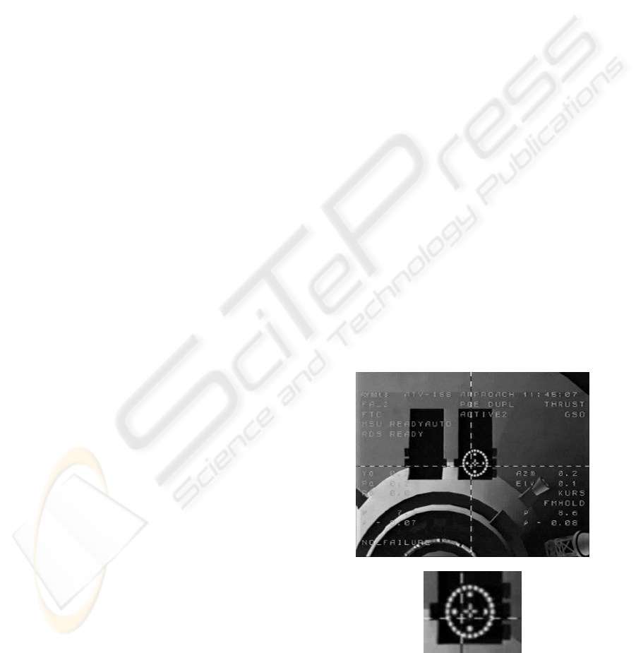
1a) Calculation of the ROI coordinates (figure 1)
on the basis of the external information (for
example, with taking into account a scene structure
or by the operator selection).
1b) Calculation of the ROI coordinates and sizes
on the basis of the information received from the
previous images processing.
a)
b)
Figure 1: An example of identification of a region of
interest in the TV camera field of view (1.а) way): а) –
total field of view, b) – a region of interest.
AUTOMATIC VISION-BASED MONITORING OF THE SPACECRAFT ATV RENDEZVOUS / SEPARATIONS
WITH THE INTERNATIONAL SPACE STATION
285
The second (preprocessing) task is solved on the
basis of the histogram analysis. This histogram
describes a brightness distribution inside the ROI.
The brightness histogram should allow the reliable
transition to the binary image. In the considered task
the brightness histogram is approximately bimodal.
The desired histogram shape is provided by the
automatic brightness and contrast control of the
image source device.
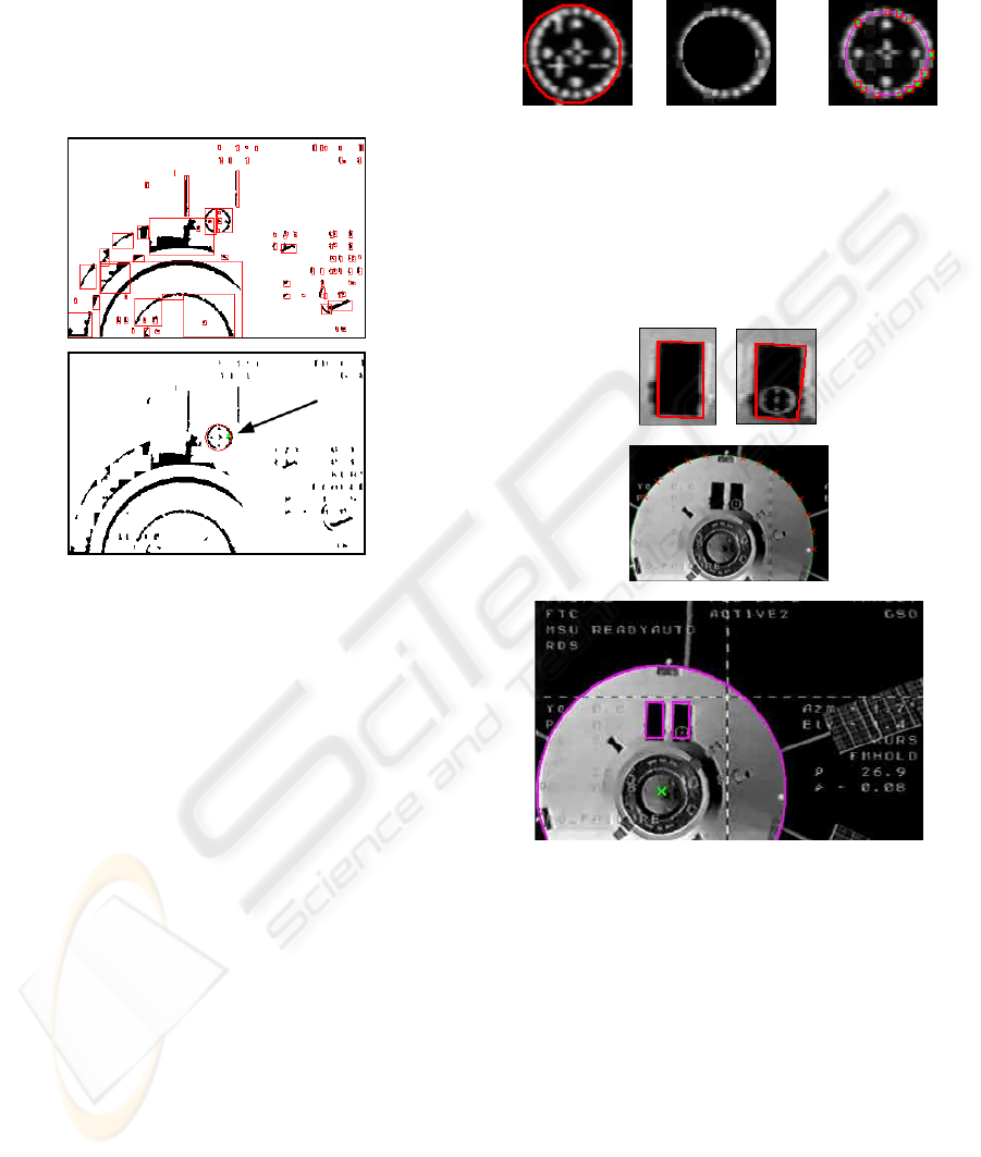
Figure 2: Coarse allocation of a target from all candidates
on a basis of the a priory information: the relative sizes of
labels and target plate and their relative location.
At the third processing stage (the task 3) the
extraction of the objects of interest is performed.
These objects are the spaceship contour, the docking
unit disk, the target cross and the target disk with
small labels. The main features are the spaceship
contour, the cross and the target labels. These
features are considered the main structured elements
of the recognized scene and used for measurement.
At features extraction both edge-based (Canny,
1986; Mikolajczyk et al., 2003) and region-based
methods are used (Sonka and Hlavac, 1999).
With accordance to such elements set the
processing of the current field image is being
performed. For example, on distances less than 15
meters are made detection of a target plate, its labels
and a cross. During such processing (figures 1, 2, 3)
the results of the previous measurements can be used
for estimation of the small area of interest position
(figure 1, below). If the previous results are not
present (for example, immediately after system
start), as area of interest is processed the full field
image. During processing among candidates for a
target image of a target it selects the most probable
candidate (figure 2). For its verification the detection
of labels and of radius of a target (figure 3) is
performed. After that the detection of a cross of a
target is performed.
a) b) c)
Figure 3: An example of allocation of an image of a target
on the basis of the coarse coordinates of a target plate and
a priory of the information on an arrangement of labels of
a target. а) - definition of area of interest on a basis a
priory of the information and found coarse location of the
plate; b) area of interest for search of labels of a target; c) -
result of allocation of labels of a target.
Figure 4: An example of allocation of edge of target boxes
and external contour of spaceship (for distance >10
meters). Top-down: extracted edges of the left and the
right boxes; contour of the spaceship; results of the frame
processing (with the marked docking unit image centre).
On distances more than 15 m a label and a cross
of a target reliably are not visible. Therefore the
detection of an external contour of the ship and a
target boxes (figure 4) is realized. Boxes of a target
allow to confirm a hypothesis about the detection of
the ship and to specify its roll position.
The fourth operation (performing of the
measurement) is very straightforward. But for this
operation it is necessary to recognize the reliable
objects results from the previous processing stages.
ICINCO 2007 - International Conference on Informatics in Control, Automation and Robotics
286

3 CALCULATION PART
Preprocessing of a frame (more exactly, a half-
frame) gives the following information:
T
– reference time of a frame (in seconds);
CC
YX ,
– real values coordinates of the center of
the cross on the target;
1
N
–number of couples of
points on the horizontal crossbar of the cross;
),,2,1(,
1
NiYX
ii
…=
– integer coordinates of
points on the top of the horizontal crossbar of the
cross;
),,2,1(,
1
NiYX
ii
…=
′
– coordinates of points
on the bottom of the horizontal crossbar of the cross;
2
N
– number of couples of points on the vertical
crossbar of the cross;
),,2,1(,
2
NiVU
ii
…=
–
coordinates of points on the left side of vertical
crossbar of the cross;
),,2,1(,
2
NiVU
ii
…=
′
–
coordinates of points on the right side of vertical
crossbar of the cross;
RYX
OO
,,
– coordinates of
the center of the circle on the target and its radius;
),,2,1(,,
33
NiBAN
ii
…=
– number of points on
the circle and their coordinates;
SSS
RYX ,,
–
coordinates of the center of the circle, which is the
station outline, and its radius (real numbers).
Here all coordinates are expressed in pixels.
Successful preprocessing a frame always gives the
values of
CC
YX ,
and
RYX
OO
,,
, but if there is an
opportunity, when appropriate
0>
k
N
, those
quantities are determined once again by original
information. Bellow we describe the calculation of
those quantities in the case when
0,0,0
321
>>> NNN
and
0=
S
R
. If
S
R
differs
from zero, the data are used in other way (see
bellow).
Determining the coordinates of the cross center.
We change the data
i
ii
Y
YY
→
′
+
2
,
i
ii
U
UU
→
′
+
2
),2,1( …=i
and get coordinates of two sequences of points,
which lie in centerlines of horizontal and vertical
crossbars of the cross. Those centerlines have
equations
1
cyax =−
(horizontal) and
2
cayx
=
+
(vertical). Here
a
,
1
c
and
2
c
are coefficients. The
form of the equations takes into account the
orthogonality of these lines. The coefficients are
determined by minimization of the quadratic form
∑∑
==
+++−−
21
1
2
2
1
2
1
)()(
N
j
jj
N
i
ii
caVUcYXa
on
21
,, cca
, i.e. by solving the linear least squares
problem. The coordinates of the cross center are
2
21
*
1 a
cac
X
C
+
+
=
,
2
21
*
1 a
acc
Y
C
+
−
=
.
Determining the radius and the center of the
target circle is realized in two stages. In the first
stage, we obtain preliminary estimations of these
quantities based on elementary geometry. In the
second stage, we solve the least squares problem
minimizing the expression
()()
∑
=
⎥
⎦
⎤
⎢
⎣
⎡
−−+−=Φ
3
1
2
22
2
N
i
OiOi
RYBXA
on
RYX
OO
,,
by Gauss-Newton method (Bard,
1974). Let its solution be
***
,, RYX
OO
. As a rule,
||
*
OO
XX −
and
||
*
OO
YY −
do not exceed 1.5
pixels. Below for simplicity of notations, we will not
use an asterisk in designations of recomputed
parameters.
3.1 Basic Geometrical Ratios
We use the right Cartesian coordinate system
321
yyCy
, which is connected with the target. The
point
C
is the center of the target circle, the axis
3
Cy
is directed perpendicularly to the circle plane
away from station, i.e. is parallel a longitudinal axis
of the Service module, the axis
+
2
Cy
intersects a
longitudinal axis of the docking device on the
Service Module. Also, we use right Cartesian
coordinate system
321
xxSx
connected with the TV
camera on the spacecraft. The plane
21
xSx
is an
image plane of the camera, the axis
3
Sx
is a camera
optical axis and directed on movement of the
spacecraft, the axis
−
2
Sx
intersects an axis of the
docking device of the spacecraft. Let
3
1,
||||
=ji
ij
a
be the
transition matrix from the system
321
xxSx
to the
system
321
yyCy
. The transition formulas are
)3,2,1(
3
1
=+=
∑
=
ixady
j
jijii
,
∑
=−= )3,2,1()( jadyx
ijiij
.
Here
321
,, ddd
are coordinates of the point S
in the system
321
yyCy
.
AUTOMATIC VISION-BASED MONITORING OF THE SPACECRAFT ATV RENDEZVOUS / SEPARATIONS
WITH THE INTERNATIONAL SPACE STATION
287

The matrix characterizes ideal docking
)1,1,1(diag|||| −−=
ij
a
. In actual docking the transition
matrix is
1
1
1
||||
12
13
23
−−
−−
−
=
ϕϕ
ϕϕ
ϕϕ
ij
a
where
32
,,
ϕ
ϕ
ϕ
are components of the vector of an
infinitesimal rotation of the system
321
xxSx
with
respect to its attitude in ideal docking. We suppose
deviations from ideal docking are small.
If any point has in the system
321
xxSx
the
coordinates
),,(
321
xxx
, its image has in the image
plane the coordinates
3
1
1
x
fx
=
ξ
,
3
2
2
x
fx
=
ξ
.
Here
f
is focal length of the camera. The
coordinates
1
ξ
and
2
ξ
, expressed in pixels, were
meant in the above description of processing a single
video frame. Let coordinates of the same point in the
system
321
yyCy
be
),,(
321
yyy
. Then
333323221311
333222111
)()()(
)()()(
adyadyady
adyadyady
f
iii
i
−+−+−
−+−+−
=
ξ
.
The coordinates of the center of the target circle
the
C in the system
321
yyCy
are
)0,0,0(
, therefore
31221
23321
ddd
ddd
fX
O
−+
+−
=
ϕϕ
ϕϕ
,
31221
13231
ddd
ddd
fY
O
−+
++
−=
ϕϕ
ϕϕ
.
In docking
31
|| dd <<
,
32
|| dd <<
, so it is
possible to use the simplified expressions
2
3
1
ϕ
f
d
fd
X
O
−−=
,
1
3
2
ϕ
f
d
fd
Y
O
+=
.
The center of the cross in the system
321
yyCy
has the coordinates
),0,0( b
. In this case under the
similar simplification, we have
2
3
1
ϕ
f
bd
fd
X
C
−
−
−=
,
1
3
2
ϕ
f
bd
fd
Y
C
+
−
= .
So
)
3
(
3
1
bdd
bdf
O
X
C
X
−
−=−
,
)
3
(
3
2
bdd
bdf
O
Y
C
Y
−
=−
.
The radius
r
of the target circle and radius R of
its image in the image plane are connected by the
ratio
3
/ dfrR =
.
The last three ratios allow to express
3
d
,
1
d
and
2
d
through R ,
OC
XX −
and
OC
YY −
. Then it is
possible to find
1
ϕ
and
2
ϕ
, having solved
concerning these angles the expressions for
OO
YX ,
or
CC
YX ,
. As to the angle
3
ϕ
, the approximate
ratio
a=
3
ϕ
takes place within the framework of
our consideration.
The processing a frame is considered to be
successful, if the quantities
ii
d
ϕ
,
)3,2,1( =i
were
estimated. As a result of successful processing a
sequence of frames, it is possible to determine
spacecraft motion with respect to the station. The
successfully processed frames are used only for
motion determination.
3.2 Algorithm for Determination of the
Spacecraft Motion
The spacecraft motion is determined in real time as a
result of step-by-step processing of a sequence of
TV images of the target. The data are processed by
separate portions.
In each portion is processed in two stages. The
first stage consists in determining the motion of the
spacecraft center of mass; the second stage consists
in determining the spacecraft attitude motion.
Mathematical model of motion is expressed by
formulas
tzzd
211
+
=
,
tzzd
432
+
=
,
tzzd
653
+=
,
tvv
211
+
=
ϕ
,
tvv
432
+
=
ϕ
,
tvv
653
+=
ϕ
.
Here
t
is time counted off the beginning of
processing the frame sequence,
i
z
and
j
v are
constant coefficients. The ratios written out have the
obvious kinematical sense. We denote the values of
the model coefficients, obtained by processing the
portion of the data with number
n
, by
)(n
i
z
,
)(n
j
v
and the functions
)(td
i
,
)(t
i
ϕ
, corresponding to
those coefficients, by
)(
)(
tD
n
i
,
)(
)(
t
n
i
Φ
.
Determining the motion consists in follows. Let
there be a sequence of successfully processed
frames, which correspond to the instants
...
321
<
<
<
ttt
. The frame with number k
corresponds to the instant
k
t
. Values of the
quantities
C
X
,
C
Y
, a ,
O
X
,
O
Y
, R , which were
found by processing this frame, are
)(k
C
X
,
)(k
C
Y
, etc.
These values with indexes
1
,,2,1 Kk …=
form the
first data portion, the value with indexes
211
,,2,1 KKKk …
+
+
=
– the second one, with
indexes
nnn
KKKk ,,2,1
11
…++=
−−
– the n -th
portion.
The first data portion is processed by a usual
method of the least squares. The first stage consists
in minimization of the functional
∑
=
=Ψ
1
1
1
)(
K
k
k
Az
,
ICINCO 2007 - International Conference on Informatics in Control, Automation and Robotics
288

+
⎥
⎥
⎦
⎤
⎢
⎢
⎣
⎡
−
+−=
2
)(
3
)(
3
)(
1
)()(
1
][ bdd
bdf
XXwA
kk
k
k
O
k
C
k
+
⎥
⎥
⎦
⎤
⎢
⎢
⎣
⎡
−
−−
2
)(
3
)(
3
)(
2
)()(
2
][ bdd
bdf
YYw
kk
k
k
O
k
C
2
)(
3
)(
3
⎥
⎥
⎦
⎤
⎢
⎢
⎣
⎡
−
k
k
d
fr
Rw
Here
)(
)(
ki
k
i
tdd =
,
T
zzzz ),,,(
621
…=
is a
vector of the coefficients, which specify the
functions
)(td
i
,
i
w
, is positive numbers (weights).
The minimization is carried out by Gauss -Newton
method (Bard, 1974). The estimation
)1(
z
of
z
and
the covariance matrix
1
P
of this estimation are
defined by the formulas
[]
)(minarg,,,
1
)1(
6
)1(
2
)1(
1
)1(
zzzzz
T
Ψ== …
,
1
1
2
1
−
= BP
σ
,
[
]
63
1
)1(
1
2
−
Ψ
=
K
z
σ
.
Here
1
B
is the matrix of the system of the
normal equations arising at minimization of
1
Ψ
. The
matrix is calculated at the point
)1(
z
.
At the second stage, the quantities
⎥
⎥
⎦
⎤
⎢
⎢
⎣
⎡
−=
)(
)(
1
)1(
3
)1(
2
)()(
1
k
k
k
O
k
tD
tfD
Y
f
α
,
⎥
⎥
⎦
⎤
⎢
⎢
⎣
⎡
+−=
)(
)(
1
)1(
3
)1(
1
)()(
2
k
k
k
O
k
tD
tfD
X
f
α
are calculated and three similar linear regression
problems
k
k
tvv
21
)(
1
+≈
α
,
k
k
tvv
43
)(
2
+≈
α
,
k
k
tvva
65
)(
+≈
),,2,1(
1
Kk …=
are solved using the standard least squares method
(Seber, 1977). We content ourselves with
description of estimating the couple of parameters
21
, vv
. We unite them in the vector
T
vvv ),(
21
=
.
The estimations
)1(
1
v
and
)1(
2
v
provide the minimum
to the quadratic form
[]
2
1
21
)(
1
1
1
)(
∑
=
−−=
K
k
k
k
tvvvF
α
.
Let
1
Q
be the matrix of this form. Then the
covariance matrix of the vector
T
vvv ],[
)1(
2
)1(
1
)1(
=
is
)2/(][
1
)1(
1
1
1
−
−
KvFQ
.
The second data portion is carried out as follows.
At the first stage, the functional
[][]
∑
+=
+−−=Ψ
2
1
1
)1(
2
)1(
2
)(
K
Kk
k
T
AzzCzzz
is minimized. Here
12
qBC
=
,
q
is a parameter,
10 ≤≤ q
. The estimation of
z
and its covariance
matrix have the form
)(minarg
2
)2(
zz Ψ=
,
1
2
2
2
−
= BP
σ
,
[]
6)(3
12
)2(
2
2
−−
Ψ
=
KK
z
σ
,
where
2
B
is the matrix of the system of the normal
equations, which arise at minimization of
2
Ψ
,
calculated at the point
)2(
z .
At the second stage, the quantities
)(
1
k
α
and
)(
2
k
α
(see above) are calculated and the estimation
of the coefficients
)2(
j
v are found. The estimation
)2(
v
provides the minimum to the quadratic form
[
]
[
]
+−−
′
=
)1(
1
)1(
2
)( vvQvvqvF
T
[]
2
1
21
)(
1
2
1
∑
+=
−−
K
Kk
k
k
tvv
α
.
Here
q
′
is a parameter,
10 ≤
′
≤ q
. Let
2
Q
be
the matrix of this form. The covariance matrix of the
estimation
)2(
v is
)2/(][
12
)2(
2
1
2
−−
−
KKvFQ
.
The third and subsequent data portions are
processed analogously to the second one. The
formulas for processing the portion with number
n
are obtained from the formulas for processing the
second portion by replacement of the indexes
expressed the portion number:
11 −→ n , n→2 .
Our choice of
n
C
and
)(z
n
Ψ
means that the
covariance matrix of errors in
OC
XX −
,
OC
YY
−
and
R is equal to ),,(diag
1
3
1
2
1
1
−−−
www .
It is easy to see that
1−
<
nn
BC
, i.e. the matrix
nn
CB
−
−1
is positive definite. The introduction of
the matrix
n
G
provides diminution of influence of
the estimation
)1( −n
z
on the estimation
)(n
z
.
Unfortunately, the matrix
n
G
is unknown. In such
situation, it is natural to take
1−
=
nn
qBC
. One has
1−
<
nn
BC
if
1
<
q
. The described choice of
n
C
means, that procession of the
n -th data portion takes
into account the data of the previous portions. The
data of the
n
-th portion are taken in processing with
the weight 1, the
)1(
−
n
-th portion is attributed the
weight
q
, the
)2(
−
n
-th portion has the weight
2
q
,
etc.
The results of processing the
n -th data portion
are represented by numbers
)(
)(
n
K
n
i
tD
, )(
)(
n
K
n
i
tΦ
),2,1;3,2,1( …
=
=
ni
. We calculate also the
quantities
2
3
2
2
2
1
ddd ++=
ρ
,
d
t
d
u
ρ
=
,
2
3
2
1
2
arctan
dd
d
+
=
α
,
3
1
arctan
d
d
=
β
.
AUTOMATIC VISION-BASED MONITORING OF THE SPACECRAFT ATV RENDEZVOUS / SEPARATIONS
WITH THE INTERNATIONAL SPACE STATION
289
The angle
α
is called a passive pitch angle, the
angle
β
is a passive yaw angle. If docking is close
to ideal (considered case), then
31
|| dd
<
<
,
32
|| dd <<
and
32
/ dd=
α
,
31
/ dd=
β
.
The angle
1
ϕ
is called an active pitch angle,
2
ϕ
is an active yaw angle,
3
ϕ
is an active roll angle.
We remind these angles have small absolute values.
Characteristics of accuracy of the motion
parameter estimations are calculated within the
framework of the least squares method. For
example, we defined above the covariance matrix
n
P
of the estimation
)(n
z
. In terms of this matrix
the covariance matrix
)(tC
w
of the vector
=
)(tw
()
12
665443221
,,,,,, Rvtvvztzzztzz
T
∈+++ …
is
calculated by formulas
T
nw
z
w
P
z
w
C
⎟
⎠
⎞
⎜
⎝
⎛
∂
∂
∂
∂
=
,
U)U,(U,diag=
∂
∂
z
w
,
00
1 t
U =
.
These formulas concern to the motion which was
found by processing the
n -th of a portion of the
data.
Knowing
)(tC
w
, it is possible to calculate the
standard deviations
)(t
ρ
σ
,
)(t
u
σ
,
)(t
α
σ
and
)(
t
β
σ
of the quantities
)(t
ρ
,
)(tu
,
)(t
α
and
)(t
β
.
The standard deviation
)(t
ρ
σ
has the form
T
w
w
C
w
⎟
⎠
⎞
⎜
⎝
⎛
∂
∂
∂
∂
=
ρρ
σ
ρ
,
T
d
dd
w
⎟
⎟
⎠
⎞
⎜
⎜
⎝
⎛
=
∂
∂
ρρρ
ρ
3
21
,0,,0,
.
The similar formulas define the others standard
deviations. The values of
ρ
,
ρ
σ
, u ,
u
σ
, etc.,
referring to the last instant of the processed data
portion, are written on the computer display.
4 EXAMPLES
The experiments with the described complex were
carried out on various samples of the initial data.
The adjustment of system on the images of the
transport ship ATV was carried out on photos of a
breadboard model of the ship in a hangar and on
rendered samples of the 3D ship model trajectories.
Other initial data were real video received from a
board of the ship "Progress". These data were used
for an estimation of reliability and correctness of the
detection of real objects, and also for the verification
of algorithms of relative movement parameters
calculation.
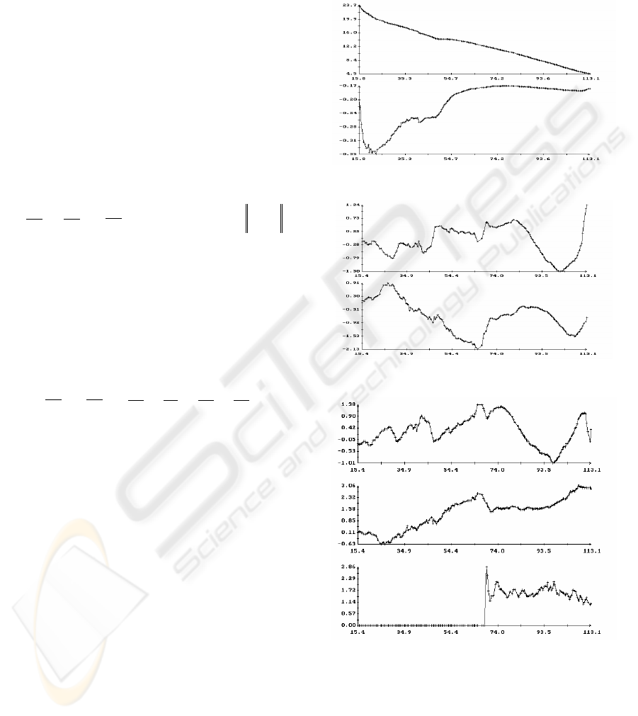
Figures 5, 6 give examples of the operation of
the described algorithm estimating the spacecraft
motion. Figure 5 contains the plots of the functions
)(t
ρ
,
)(tu
,
)(t
α
and
)(t
β
and
)(t
i
ϕ
)3,2,1( =i
.
On
)(t
ρ
and
)(tu
plots the scale on a vertical axis
differs on 2 order.
ρ
(m), u (m/s)
t (s)
β
α
,
(deg.)
t (s)
321
,,
ϕϕϕ
(deg.)
t (s)
Figure 5: Results of the determination of the spacecraft
motion in docking approach.
Figure 6 presents the plots of the standard
deviations
)(t
ρ
σ
,
)(t
u
σ
,
)(t
α
σ
,
)(t
β
σ
. The values
of all these functions were calculated at the last
instants of processed data portions. These values
ICINCO 2007 - International Conference on Informatics in Control, Automation and Robotics
290
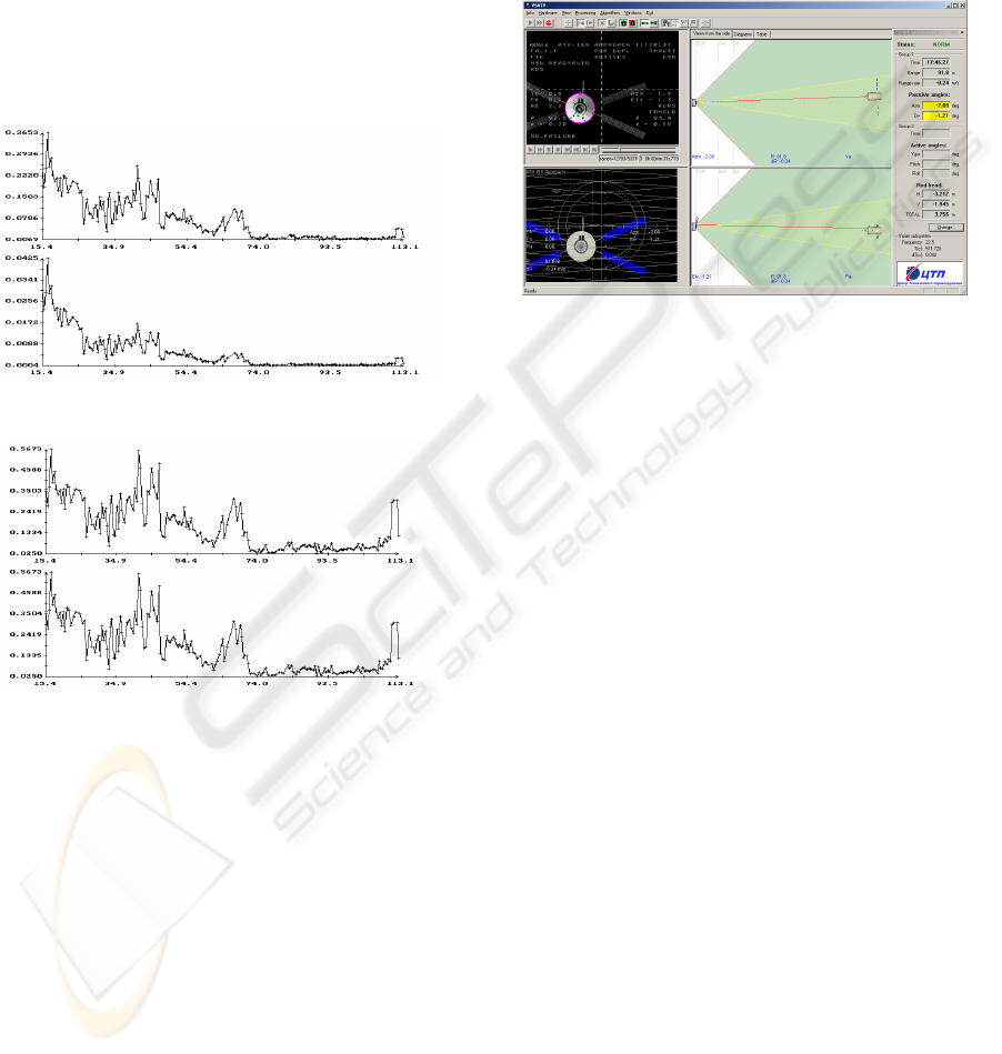
were shown by marks. Each portion contained 10
instants with measurements:
10
1
=−
−nn
KK
. For
clearness, the markers were connected by segments
of straight lines, therefore presented plots are broken
lines. Only the vertexes of these broken lines are
significant. Their links are only interpolation, which
is used for visualization and not always exact. As it
is shown in figure 6, the spacecraft motion on the
final stage of docking was defined rather accurately.
Figure 7 shows an example of the basic screen of
the main program of a complex.
ρ
σ
(m),
u
σ
(m/s)
t (s)
βα
σ
σ
, (deg.)
t (s)
Figure 6: Accuracy estimations for the motion presented
on Figure 5.
5 CONCLUSION
The described complex is being prepared for the use
as a means allowing the ground operators to receive
the information on the motion parameters of the
spacecraft docking to ISS in real time.
The most essential part of this information is
transferred to the Earth (and was always transferred)
on the telemetering channel. It is also displayed on
the monitor. However this so-called regular
information concerns the current moment and
without an additional processing can’t give a
complete picture of the process. Such an additional
processing is much more complicated than the
organizational point of view and more expensive
than processing the video image. It is necessary to
note, that the estimation of kinematical parameters
of the moving objects on the video signal, becomes
now the most accessible and universal instrument of
solving such kind of problems in situations, when
the price of a failure is rather insignificant.
Figure 7: Main screen of the VSATV program.
REFERENCES
Boguslavsky A.A., Sazonov V.V., Smirnov A.I., Sokolov
S.M., Saigiraev K.S., 2004. Automatic Vision-based
Monitoring of the Spacecraft Docking Approach with
the International Space Station. In Proc. of the First
International Conference on Informatics in Control,
Automation and Robotics (ICINCO 2004), Setúbal,
Portugal, August 25-28, 2004, Vol. 2, p.79-86.
Chi-Chang, H.J., McClamroch, N.H., 1993. Automatic
spacecraft docking using computer vision-based
guidance and control techniques. In Journal of
Guidance, Control, and Dynamics, vol.16, no.2:
pp. 281-288.
Casonato, G., Palmerini, G.B., 2004. Visual techniques
applied to the ATV/ISS rendezvous monitoring. In
Proc. of the IEEE Aerospace Conference, vol. 1,
pp. 619-625.
Canny, J. 1986. A computational approach to edge
detection. In IEEE Trans. Pattern Anal. and Machine
Intelligence, 8(6): pp. 679-698.
Mikolajczyk, K., Zisserman, A., Schmid, C., 2003. Shape
recognition with edge-based features. In Proc. of the
14th British Machine Vision Conference
(BMVC’2003), BMVA Press.
Sonka, M., Hlavac, V., Boyle, R. 1999. Image Processing,
Analysis and Machine Vision. MA: PWS-Kent.
Bard, Y., 1974. Nonlinear parameter estimation.
Academic Press, New York.
Seber, G.A.F., 1977. Linear regression analysis. John
Wiley and Sons, New York.
AUTOMATIC VISION-BASED MONITORING OF THE SPACECRAFT ATV RENDEZVOUS / SEPARATIONS
WITH THE INTERNATIONAL SPACE STATION
291
