
THE HEAT EQUATION AND THE FRENET FORMULAS FOR
DIGITAL CURVES
Sheng-Gwo Chen, Mei-Hsiu Chi
Department of Applied Mathematics, National Chia-Yi University, Taiwan
Department of Mathematics, National Chung-Cheng University, Taiwan
Jyh-Yang Wu
Department of Mathematics, National Chung-Cheng University, Taiwan
Keywords: Digital curves, heat equation, the Frenet formulas.
Abstract: In this note we shall discuss the heat equation and the eigenvalue problem for digital curves in the 3D
Euclidean space. First, we shall introduce the derivative of a function along a digital curve by the weighted
combination method. Then, we can define the Laplace of a function on a digital curve. The Frenet formulas
for digital curves will also be discussed. Numerical simulations show our method will provide good
estimations for the curvature and torsion.
1 INTRODUCTION
An ordered set of points },,2,1|{
3
kiRpC
i
⋅⋅⋅=∈=
is called a digital curve in the 3D Euclidean space
3
R . The digital curves can be obtained by the
discretization of regular curves or from digital
images. Understanding the geometric and
differential properties of digital curves is an
important topic in CAD or CAGD. In particular, the
curvature or the heat flow on a regular curve C in the
3D Euclidean space are important differential
invariants in the theory of space curves and its
applications to image processing and computer
graphics. The curvature and torsion are determined
by the differential of the tangent vectors and the
binormal vectors of the curve
C .
In this paper we shall discuss a differential
theory for digital curves in the 3D Euclidean space.
We shall discuss the derivative of a function along a
digital curve by the weighted combination method.
We shall use the centroid weights in our algorithms.
These weights were first proposed in (Chen and Wu,
2004) to improve Taubin’s method for the estimation
of curvatures on a triangular mesh in the 3D
Euclidean space. Then, we shall investigate the heat
flow and the eigenvalue problem on digital curves.
In section four, we shall discuss the moving frame of
a digital curve and obtain the discrete Frenet
formulas. This method fits perfectly with the
proposal given in (Rosenfeld and Klette, 2002)
about the field of digital geometry. Usually, the
accurate estimation of curvatures at vertices of a
digital curve plays as the first step for many
applications such as simplification, smoothing,
subdivision, visualization and image processing, etc.
Our estimation is simple and very accurate as we
shall illustrate them in the numerical simulations.
2 THE LOCAL THEORY FOR
REGULAR CURVES
In this section we first recall some basic notions and
results about the local theory of smooth regular
curves in the 3D Euclidean space
3
R . See (do Carmo,
1976) for details. Consider a smooth regular curve
))(),(),(()( szsysxsc
=
,
],0[ ls
∈
with arc length
parameter
s
.
Given a function
)(sf on )(sc , we can define the
Laplacian
)(sf
Δ
of f by
)()(
2
2
sf
ds
d
sf =Δ
.
(2-1)
97
Chen S., Chi M. and Wu J. (2007).
THE HEAT EQUATION AND THE FRENET FORMULAS FOR DIGITAL CURVES.
In Proceedings of the Second International Conference on Computer Graphics Theory and Applications - GM/R, pages 97-102
DOI: 10.5220/0002072900970102
Copyright
c
SciTePress

The eigenvalue problem is given by
The heat equation for the function
),( tsu is given by
Next we discuss the curvature and torsion of the
regular curve
))(),(),(()( szsysxsc = in
3
R
with arc
length parameter
s
. The tangent vector
))('),('),('()(' szsysxsc = , denoted by )(st
r
, is a unit
vector since s is the arc length parameter. The
number
)()(' sst
κ
=
r
is called the curvature of c at
s
.
At points where
0)( ≠s
κ
, a unit vector )(sn
r
in the
direction
)(' st
r
is well-defined by the
equation
)()()('
snsst
r
r
κ
=
. The vector
)(sn
r
is
perpendicular to
)(st
r
and is called the normal vector
of
c at
s
. The plane determined by the unit tangent
vector )(
st
r
and normal vectors
)(sn
r
is called the
osculating plane of
c at
s
. At points where 0)(
=
s
κ
,
the normal vector and hence the osculating plane are
not defined. In what follows, we shall restrict
ourselves to curves parametrized by arc length
with
0)( ≠s
κ
for all ],0[ ls ∈ . The unit
vector
)()()( snstsb
r
r
r
×= is normal to the osculating
plane and will be called the binormal vector of
c at
s
.
The number )(' sb
r
measures the rate of change of
the neighboring osculating planes of
C at
s
. That is,
)(' sb
r
measures how rapidly the curves pulled
away from the osculating plane of
c at
s
in a
neighborhood of
s
. The Frenet formulas are
These Frenet formulas form a system of ordinary
differential equations (ODE’s) for the vectors
)(st
r
,
)(sn
r
and )(sb
r
. We shall call the matrix
the Frenet matrix of the curve c at s.
3 A DISCRETE HEAT EQUATION
FOR A DIGITAL CURVE
In this section we shall introduce a discrete heat
equation for a digital curve in the 3D Euclidean
space
3
R . A digital curve C in the 3D Euclidean
space is an ordered set of points
}.,,2,1:{
3
kiRpC
i
⋅⋅⋅=∈=
Consider a
function
f on the digital curve C . We can define the
discrete derivative of the function
f by:
when the point
i
p is an interior point. When
i
p is a
boundary point i.e.,
0
=
i or
k
, we take the one-side
derivative:
and
Indeed, when we know how to compute the
derivatives of functions on a digital curve
C , we can
also compute their higher order derivatives. From
the experience given in (Chen and Wu, 2004), (Chen
and Wu, 2005) and (Wu, Chen and Chi 2005), we
shall use the centroid weights for the
weights
1
ω
and
2
ω
. Namely, for the digital
curve
},,2,1:{
3
kiRpC
i
⋅⋅⋅=∈=
, we have at the
point
i
p
⎪
⎪
⎪
⎪
⎪
⎪
⎩
⎪
⎪
⎪
⎪
⎪
⎪
⎨
⎧
−
+
−
−
=
−
+
−
−
=
+−
+
+−
−
)
11
(
1
)
11
(
1
2
1
2
1
2
1
2
2
1
2
1
2
1
1
iiii
ii
iiii
ii
pppp
pp
pppp
pp
ω
ω
(3-4)
ff
λ
=Δ .
(2-2)
uu
t
Δ=
∂
∂
.
(2-3)
)()()(' snsst
r
r
κ
=
(2-4)
)()()()()(' sbsstssn
r
r
r
τκ
−−=
(2-5)
)()()(' snssb
r
r
τ
=
(2-6)
⎟
⎟
⎟
⎠
⎞
⎜
⎜
⎜
⎝
⎛
−−=
0)(0
)(0)(
0)(0
)(
s
ss
s
sF
τ
κτ
κ
(2-7)
ii
ii
ii
ii
i
pp
pfpf
pp
pfpf
pf
dx
d
−
−
+
−
−
=
+
+
−
−
1
1
2
1
1
1
)()(
)()(
)(
ω
ω
(3.1)
12
12
1
)()(
)(
pp
pfpf
pf
dx
d
−
−
=
(3-2)
1
1
)()(
)(
−
−
−
−
=
kk
kk
k
pp
pfpf
pf
dx
d
(3-3)
GRAPP 2007 - International Conference on Computer Graphics Theory and Applications
98

From this we can consider the discrete heat equation
on
C for a function ),( tpu
i
:
If we consider the vector
T
i
tputv )),(()( = in
k
R , a
direct computation of (3-4) will lead to a system of
ODE’s:
where
)(
ijk
aA = is a kk × matrix with constant
ij
a .
The constant
ij
a depends only on the points on C .
From the theory of differential equations, the
solution for
T
i
tputv )),(()( = will have the form:
)0()( vetv
k
tA
=
(3-7)
with the initial value
T
i
puv ))0,(()0( = . The matrix
k
tA
e
can be computed from the formula
∑
∞
=
=
0
!
)(
n
n
k
tA
n
tA
e
k
(3-8)
When the matrix
k
A
is symmetric, it is
diagonalizable and one can find an orthogonal
kk × matrix
Q
and a diagonal kk × matrix
D
such
that
QAQD
k
T
=
. Note that the column vectors of the
orthogonal matrix
Q are eigenvectors of
k
A and the
diagonal matrix
)(
j
diagD
λ
= is given by the
corresponding eigenvalues of
k
A
. In this case the
solution
)(tv can be obtained from
)0()()( QvediagQtv
j
t
T
λ
=
(3-9)
It can be shown easily that the proposed discrete
heat density converges to the real heat density if a
smooth curve is sampled finer and finer. This is also
true for the curvature and torsion as one can see
from the numerical simulations in section 5.
To illustrate our ideas, we consider the digital
curve to be uniformly distributed and closed.
Namely, the digital curve
},,1,0:{
3
kiRpC
i
⋅⋅⋅=∈=
has constant distances
1+
−=
ii
pph for all
1,,1,0 −⋅⋅⋅= ki
and
k
pp
=
0
,
An easy computation gives the
kk
×
matrix
)(
4
1
2
ijk
a
h
A =
with
2−=
ii
a
,
1=
ij
a
when
2=− ji )mod(k
; otherwise,
0=
ij
a
.
In particular, the matrix
k
A
is symmetric and
diagonalizable.
Therefore to study the discrete heat equation
(3-5), we are led to the matrix eigenvalue problem
To obtain the eigenvalues and their corresponding
eigenvectors of
k
A
, we can transform the
matrix
k
A
into a double stochastic matrix
k
B
by
where
k
I
is the
kk
×
identity matrix. This
means that the double stochastic
matrix
)(
ijk
bB
=
has
2
1
=
ij
b
when
2=− ji )mod(k
;
otherwise
0
=
ij
b
.
When
k is odd, we can permute the order of the
coordinates by
1,,4,2,,,3,1 −kk LL to obtain a
new double stochastic matrix
)(
ijk
cC =
with
has
2
1
=
ij
c
when
1=− ji )mod(k
; otherwise,
0
=
ij
c
:
⎥
⎥
⎥
⎥
⎥
⎥
⎥
⎥
⎥
⎥
⎥
⎥
⎥
⎥
⎦
⎤
⎢
⎢
⎢
⎢
⎢
⎢
⎢
⎢
⎢
⎢
⎢
⎢
⎢
⎢
⎣
⎡
=
0
2
1
000
2
1
2
1
0
2
1
000
0
2
1
0000
0000
2
1
0
000
2
1
0
2
1
2
1
000
2
1
0
L
L
O
MMOOOMM
O
L
L
C
We have
QPBPC
k
T
k
=
for some permutation
matrix
P
. We note that the graph associated with the
double stochastic matrix
k
C
is a k-polygon (see
Figure 1).
Figure 1: k-polygon.
When
k
is even, we can permute the order of the
coordinates by
kk ,,4,2,1,,3,1 LL
−
and obtain a
u
x
u
t
2
2
∂
∂
=
∂
∂
.
(3-5)
)()( tvAtv
dt
d
k
=
(3-6)
vvA
k
λ
=
.
(3-10)
kkk
IAhB +=
2
2
(3-11)
1
−
k
1
3
4
k
2
THE HEAT EQUATION AND THE FRENET FORMULAS FOR DIGITAL CURVES
99

new double stochastic matrix
k
D
. Indeed, the
matrix
k
D
decomposes into two blocks:
⎥
⎥
⎦
⎤
⎢
⎢
⎣
⎡
=
2
2
0
0
k
k
k
C
C
D
(3-12)
where
2/k
C
is as above. The graph associated with the
double stochastic matrix
k
D
is two separated
(k/2)-polygons (see Figure 2).
This gives that the eigenvalues and their
corresponding eigenvectors of
k
D
can be obtained
from those of the double stochastic matrix
2/k
C
. The
double stochastic matrix
n
C
has the eigenvalues
)/2cos( nj
j
π
λ
=
,
1,...,1,0 −
=
nj
.
(3-13)
See (Bjorck and Golub, 1997). Every eigenvalue
of the matrix
n
C
has multiplicity 2 except the
eigenvalue
1 , and if n is even also 1 . Therefore,
when
k is odd, the number
j
λ
is also the eigenvalue
of the double stochastic matrix
k
B
.In turn, the
matrix
k
A
has the eigenvalues:
)1)/2(cos(
2
1
2
−= nj
h
j
πλ
,
1,...,1,0 −= kj
.
(3-14)
Every eigenvalue of the matrix
k
A
has multiplicity 2
except the eigenvalue
0 .
When
k is even, the matrix
k
D
has the eigenvalues
)/4cos( kj
j
π
λ
=
,
1,...,1,0 −
=
kj
.
(3-15)
Figure 2: (k/2)-polygons.
Every eigenvalue of the matrix
k
D
has
multiplicity
4 except the eigenvalue1 , and if
2
k
is even also
1 . When
2
k
is odd, the eigenvalue1
has multiplicity2. Hence the matrix
k
A
has the
eigenvalues
4 DISCRETE FRENET
FORMULAS FOR A DIGITAL
CURVE
In this section we shall propose an algorithm to
develop a discrete Frenet matrix for a digital curve.
Recall that a digital curve
C in the 3D Euclidean
space is an ordered set of points
}.,,2,1:{
3
kiRpC
i
⋅⋅⋅=∈= To define the tangent
vector
i
t
r
and the normal vector
i
n
r
and the binormal
vector
i
b
r
of the digital curve C at the point
i
p is the
first step to develop a geometric theory for digital
curves. To handle this, we need to formulate the
concept of the derivative of a vector field defined on
a digital curve
C .
Consider a point
i
p in the digital curve C . We can
define the tangent vector
i
t
r
of C at the point
i
p by
where
1
ω
and
2
ω
are the centroid weights given in
(3-3). Now the normal vector
i
n
r
can be computed as
follows
: First we compute the derivative
'
i
t
r
of the
tangent field
i
t
r
of C at the point
i
p by
ii
ii
ii
ii
i
pp
tt
pp
tt
t
−
−
+
−
−
=
+
+
−
−
1
1
2
1
1
1
'
rr
r
r
r
ωω
.
(4-2)
Note that the vector
'
i
t
r
may not be perpendicular
to the tangent vector
i
t
r
. We can define the curvature
i
κ
and the normal vector
i
n
r
of the digital curve C at
i
p by
As usual, the binormal vector
i
b
r
of the digital
curve
C at
i
p can be defined by
iii
ntb
r
r
r
×= . Next
we consider the torsion
i
τ
of the digital
curve
C at
i
p via the derivative of the binormal
vector field
i
b
r
.
)1)/4(cos(
2
1
2
−= kj
h
j
πλ
,
1,...,1,0 −= kj
.
(3-16)
ii
ii
ii
ii
ii
ii
ii
ii
i
pp
pp
pp
pp
pp
pp
pp
pp
t
−
−
+
−
−
−
−
+
−
−
=
+
+
−
−
+
+
−
−
1
1
2
1
1
1
1
1
2
1
1
1
)(
ωω
ωω
r
(4-1)
⎪
⎪
⎩
⎪
⎪
⎨
⎧
⋅−
⋅−
=
⋅−=
iiii
iiii
i
iiiii
tttt
tttt
n
tttt
rrrr
rrrr
r
r
r
r
r
)(
))((
)(
''
''
''
κ
.
(4-3)
1
2
2
k
k
1−k
1
2
−
k
1
2
+
k
2
2
+
k
GRAPP 2007 - International Conference on Computer Graphics Theory and Applications
100

We have
and the torsion
i
τ
can be defined by
iii
nb
r
r
⋅=
'
τ
. The
discrete version of the Frenet formulas will then
have the form
:
where the coefficients
ij
a may not be zero. This is
due to the discrete effect of the digital curve
C . We
define the discrete Frenet matrix of the digital
curve
C at
i
p to be the 33
×
matrix:
where
ij
a is given by equations (4-5), (4-6) and
(4-7).
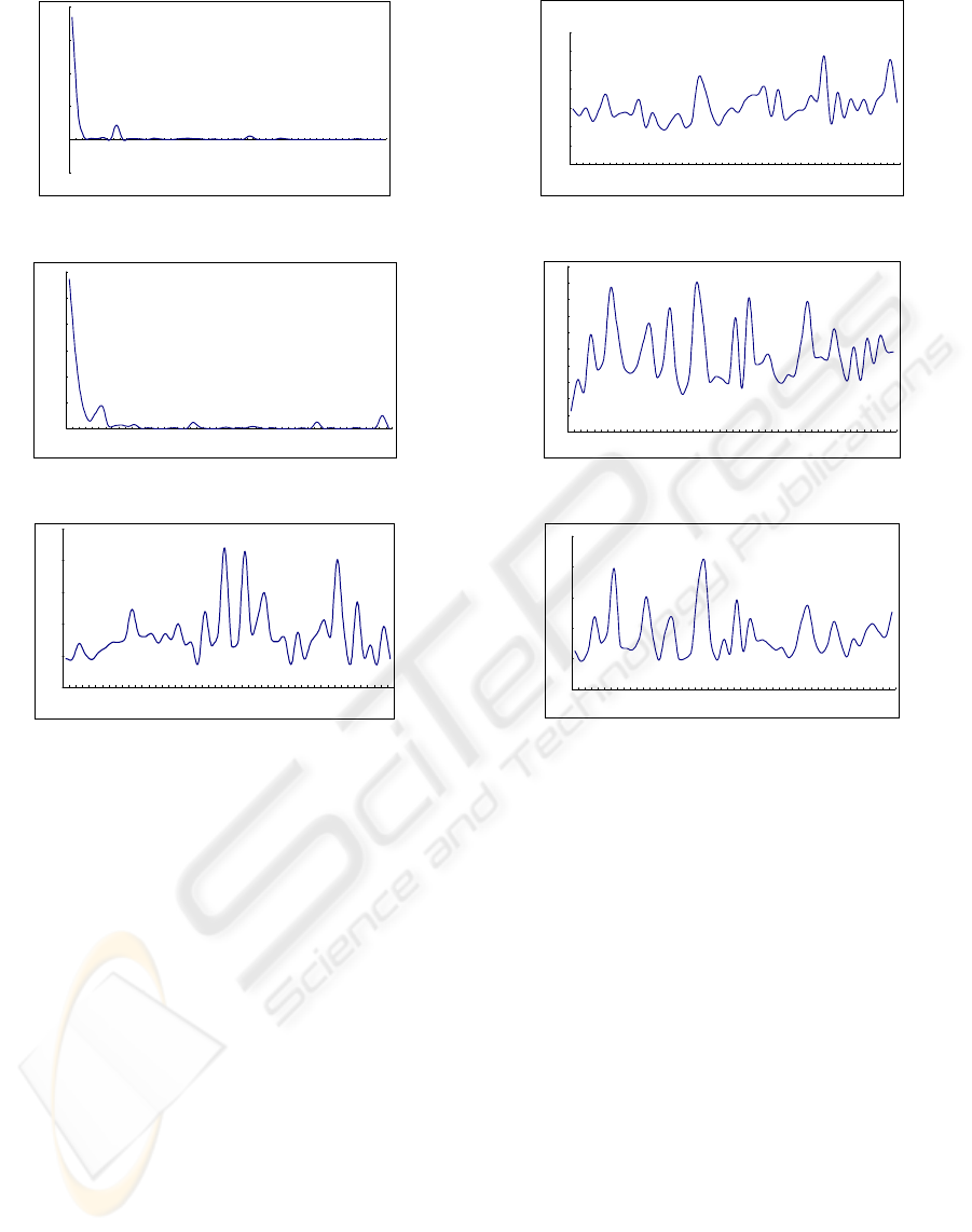
5 NUMERICAL SIMULATIONS
In this section, we will find the Frenet matrices of
the closed curves ( without boundary points ) and the
open curves ( with two boundary points ). For closed
curves, we choose the ellipses and
2
C
Bezier curves.
For open curves, we choose the helix
),sin,cos()(
c
b
c
s
a
c
s
atc =
(5-1)
with 0, >ba and
22
bac += . We shall compare
the error between the exact Frenet matrix and our
estimated discrete Frenet matrix by
||||
||||
RF
FRF
Error
−
=
(5-2)
where
R
F
is the exact Frenet matrix of the given
regular curve and
•
is the norm of matrix. We will
digitize these curves by two different kinds of
partitions -- uniform and non-uniform partitions. In
figures 3 to 8, the x-axis presents the number of
points of digital curves and the y-axis gives the
average of errors. We test 1,000 different random
curves in each partition for different size of points
and compute their average.
In figures 3 and 4, we show the numerical results
of closed curves and helix by uniform partitions.
From these results, the discrete Frenet matrix
approximates to the exact Frenet matrix very quickly.
In figures 5 and 8, we test the helix with uniform or
non-uniform partitions at the interior points and the
boundary points. These numerical simulations show
that our discrete method is very stable.
ACKNOWLEDGEMENTS
This work is partially supported by NSC, Taiwan.
We also thank Professor Chen-Yao Lai for helpful
discussions about the eigenvalue problem.
REFERENCES
Bjorck, A. Golub, G. H., 1977. Eigenproblems for matrices
associated with periodic boundary conditions. SIAM
Review Vol. 19, No. 1
Chen, S.-G.., Wu, J.-Y., 2004. Estimating normal vectors
and curvatures by centroid weights. Computer Aided
Geometric Design, 21, pp. 447-458.
Chen, S.-G.., Wu, J.-Y., 2005. A geometric interpretation
of weighted normal vectors and application.
Proceeding of the IEEE Computer Society Conference
on Computer Graphics, Imaging and Visualization,
New Trends, pp.422-425.
do Carmo, M., 1976. Differential Geometry of curves and
surfaces. Prentice Hall, Englewood Cliffs, NJ.
Rosenfeld, A. Klette, R. 2002. Digital geometry.
Information Sciences 148,p 123-127
Wu, J.-Y., Chen, S.-G. and Chi, M.-H., 2005. A simple
effective method for curvatures estimation on
triangular meshes, Technical Report WU02, NCCU,
Department of Mathematics.
ii
ii
ii
ii
i
pp
bb
pp
bb
b
−
−
+
−
−
=
+
+
−
−
1
1
2
1
1
1
'
r
r
r
r
r
ωω
(4-4)
iiii
ntat
r
rr
κ
+=
11
'
(4-5)
iiii
banatan
r
r
r
r
232221
'
++=
(4-6)
iiiii
bantab
r
r
r
r
3331
'
++=
τ
(4-7)
⎟
⎟
⎟
⎠
⎞
⎜
⎜
⎜
⎝
⎛
=
333231
232221
1211
0
aaa
aaa
aa
F
(4-8)
THE HEAT EQUATION AND THE FRENET FORMULAS FOR DIGITAL CURVES
101
uniform and closed curves
-0.05
0
0. 05
0.1
0. 15
0.2
10 30 50 70 90 110 130 150 170 190 210 230 250 270 290 310 330 350 370 390 410 430 450470490
number of poi nts
error of Frenet matrix
Figure 3: Closed curves with uniform partitions.
heli x(uni form and interi or poi nts )
0
0.0005
0.001
0.0015
0.002
0.0025
0.003
10 30 50 70 90 110 130 150 170 1 90 210 230 250 270 290 310 330 350 370 390 410 430 450470490
number of poi nts
error of Frenet matrix
Figure 4: Interior points with uniform partitions.
nonunif orm and cl osed curve
0
0.05
0.1
0.15
0.2
0.25
1
0
3
0
5
0
7
0
9
0
1
1
0
1
3
0
1
5
0
1
7
0
1
9
0
2
1
0
2
3
0
2
5
0
2
7
0
2
9
0
3
1
0
3
3
0
3
5
0
3
7
0
3
9
0
4
1
0
4
3
0
4
5
0
4
7
0
4
9
0
number of poi nts
error of Frenet matrix
Figure 5: Closed curves with non-uniform partitions.
heli x ( uniform and boundary poi nts)
0
0.2
0.4
0.6
0.8
1
1.2
1.4
1
0
3
0
5
0
7
0
9
0
1
1
0
1
3
0
1
5
0
1
7
0
1
9
0
2
1
0
2
3
0
2
5
0
2
7
0
2
9
0
3
1
0
3
3
0
3
5
0
3
7
0
3
9
0
4
1
0
4
3
0
4
5
0
4
7
0
4
9
0
number of points
error of Frenet matrix
Figure 6: Boundary points with uniform partitions.
helix( nonuni form and interi or points)
0
0.1
0.2
0.3
0.4
0.5
0.6
0.7
0.8
0.9
1
10 30 50 70 90 110 130 1 50 170 190 210 230 250 2 70 290 310 3 30 350 370 390 410 4 30 450 4 70 490
number of points
error of Frenet matrix
Figure 7: Interior points with non-uniform partitions.
heli x(nonuniform and boundary poi nts)
0
0.5
1
1.5
2
2.5
10 30 50 70 90 110 130 150 170 190 210 230 250 270 290 310 330 350 370 390 410 430 450470490
number of poi nts
error of Frenet matrix
Figure 8: Boundary points with non-uniform partitions.
GRAPP 2007 - International Conference on Computer Graphics Theory and Applications
102
