
COMPARISON OF THREE NEURAL NETWORK CLASSIFIERS
FOR APHASIC AND NON-APHASIC NAMING DATA
Antti J¨arvelin
Department of Computer Sciences, University of Tampere, FIN-33014 University of Tampere, Finland
Keywords:
Neural networks, classification, aphasia, anomia, naming disorders.
Abstract:
This paper reports a comparison of three neural network models (Multi-Layer Perceptrons, Probabilistic Neu-
ral Networks, Self-Organizing Maps) for classifying naming data of aphasic and non-aphasic speakers. The
neural network classifiers were tested with the artificial naming data generated from confrontation naming data
of 23 aphasic patients and one averaged control subjet. The results show that one node MLP neural network
performed best in the classification task, while the two other classifiers performed typically 1 - 2 % worse
than the MLP classifier. Although the differences between the different classifier types were small, these re-
sults suggests that a simple one node MLP classifier should be preferred over more complex neural network
classifiers when classifying naming data of aphasic and non-aphasic speakers.
1 INTRODUCTION
Aphasia is a language impairment following left
hemisphere damage. Aphasic patients have defect
or loss of production or receptive aspects of written
or spoken language (Harley, 2001). The most com-
mon symptom of aphasia is anomia, the impairment
in word retrieval, which has devastating effects on pa-
tients ability to carry on meaningful and effective con-
versation (Raymer and Rothi, 2002).
The language capabilities of the aphasic patients
are tested with standardized aphasia examination pro-
cedures, such as Boston Diagnostic Aphasia Exam-
ination (Goodglass and Kaplan, 1983) (in English
speaking countries) or Aachen Aphasia Test (Huber
et al., 1984) (in German speaking countries). An inte-
gral part of these tests is a picture confrontation nam-
ing task, where a subject is to name (i.e., say aloud)
single pictures. The picture naming task is used, be-
cause picture naming process involves all the major
processing stages of speech production (Laine et al.,
1992). Thus, picture naming task may more clearly
reveal the underlying mechanism and nature of pa-
tient’s anomia than the plain analysis of free speech
would (Dell et al., 1997; Cuetos et al., 2002).
Examples of common error types encountered in
the naming test include semantic errors (“cat” →
“dog”), formal errors (“cat” → “mat”), nonword er-
rors (“cat” → “tat”), mixed errors, where the response
is semantically and phonologically related to the tar-
get (“cat” → “rat”) and finally unrelated word errors
where no semantic or phonological relationship can
be found between the target and produced word.
The goal of the current study was to investi-
gate the suitability of neural network classifiers for
separating healthy individuals from aphasic patients.
Three neural network classifiers, Multi-Layer Per-
ceptrons (MLP) (Haykin, 1999), Probabilistic Neural
Networks (PNN) (Specht, 1990), and Self-Organizing
Maps (SOM) (Kohonen, 1998), were compared for
the classification of aphasic and non-aphasic naming
data. The performance of the classifiers were com-
pared using the aphasic naming data reported by Dell
et al. (1997) which was artificially augmented to suit
better for the neural network classifiers.
To our knowledge this kind of research has not
been previously reported. For example, Axer et al.
(2000) used a MLP classifier and k-nearest neighbor
classifier recognize patients’ aphasia type with their
quite large data set. However, their data set did not
contain control data from healthy subjects and thus it
cannot be used in the current study.
186
J
¨
arvelin A. (2008).
COMPARISON OF THREE NEURAL NETWORK CLASSIFIERS FOR APHASIC AND NON-APHASIC NAMING DATA.
In Proceedings of the First International Conference on Health Informatics, pages 186-190
Copyright
c
SciTePress

2 MATERIALS AND METHODS
2.1 Materials
To compare the classifiers, aphasic naming data from
Dell et al. (1997) was used (see Table 1). The data
set contains six attributes describing the Philadelphia
Naming Test (PNT) (Roach et al., 1996) results of the
subjets: correct answers, semantic errors, formal er-
rors, nonword errors, mixed errors and unrelated word
errors. The original data also contained a category
for all other miscellaneous errors, but it was excluded
from the current study as redundant. The exclusion
however explains why the error distributions of the
patients rarely sum up to 1.
The data set of Dell et al. is quite small as it only
contains naming performances of 23 aphasic patients
and an averaged naming distribution of 60 healthy
control subjects. Therefore, the data set was aug-
mented to be able to use the neural network classifiers
successfully for the task.
The data was augmented with the following pro-
cedure using the naming distributions of Table 1 as a
basis of data generation.
1. First 23 artificial control subjects were generated
from the averaged control subject and then the
generated control subjects and the 23 original pa-
tient cases were merged producing the base set of
46 subjects.
2. From the base set 10 × 10 cross-validation sets
were prepared.
3. Finally, the partitions of the cross-validation sets
were augmented so that the total size of the cross-
validation sets were 1000 cases. Thus, each pa-
tient and generated control subject served approx-
imately 22 times as a seed for data generation.
The first part of the data generation ensures an equal
class distribution between the healthy and patient
data. It also ensures that there will be more varia-
tion in the generated healthy data than there would be
if only the average control subject had been used as
the seed for all generated healthy data. The second
and third parts ensure that during cross-validation the
test and validation sets always contain cases generated
from the different seeds than the cases in the training
set making the cross-validation process more robust.
The values of the variables for each generated test
case were calculated as follows. Let v
i
be the value
of the ith variable of the seed, σ(v
i
) the standard de-
viation of variable v
i
and N(a, b) normal distribution
with mean a and standard deviation b. The value v
′
i
of
the ith variable of the artificial subject was calculated
with
v
′
i
= |v
i
+ N(0, 0.1σ(v
i
))|. (1)
Applying (1) in the data generation produces a
cloud of artificial subjects centered around the seed.
The absolute value is taken in (1) in order to avoid
negative values for the generated variables. Different
scaling factors of the variables’ standard deviations
were experimented, and 0.1 was found to be the most
appropriate one. A greater scaling factor would have
dispersed the generated cloud around the center too
much and the smaller would have resulted too com-
pact clouds.
2.2 Methods
The neural network classifiers were compared gener-
ating ten data sets with the procedure described in the
previous section. Ten data sets were used to smooth
the differences between the generated data sets. Each
classifier was examined by running a 10× 10 cross-
validation (Duda et al., 2001) for each data set. The
differences between the classifiers were compared by
calculating average classification accuracy (ACC) for
each classifier over the ten cross-validated data sets.
The total classification accuracy for a classifier is
given by
ACC = 100·
∑
C
c=1
tp
c
∑
C
c=1
p
c
%, (2)
where tp
c
denotes the number of true positive clas-
sifications and p
c
the size of the class c. For more
detailed evaluation also true positive rates (TPR) and
positive predictive values (PPV) were calculated for
the both classes. The true positive rate for class c is
given by
TPR
c
= 100·
tp
c
p
c
%, (3)
and the positive predictive value with
PPV
c
= 100·
tp
c
tp
c
+ f p
c
%, (4)
where f p
c
denotes the number of false positive clas-
sifications of the class c. The statistical significance
of the differences between the classifiers was tested
with Friedman test (Connover, 1999) over the classi-
fication accuracies.
For MLP, sigmoid activation function was used
as network’s transfer function. The networks were
trained using Levenberg-Marquardt optimized batch
mode backpropagation algorithm. To prevent over fit-
ting a separate validation set (chosen from the cross-
validation set) was used for early stopping during
the training. The networks were trained at most 100
epochs, but typically less than 100 epochs were used,
since the validation set brought the algorithm into
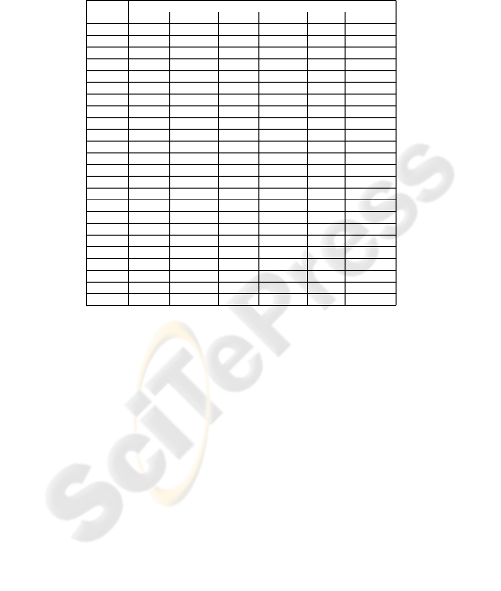
Table 1: The proportional naming distributions of 23 aphasic patients and an averaged control subject tested with PNT reported
by Dell et al. (1997).
Naming response
Patient Correct Semantic Formal Nonword Mixed Unrelated
W.B. 0.940 0.020 0.010 0.010 0.010 0.000
T.T. 0.930 0.010 0.010 0.000 0.020 0.000
J.Fr. 0.920 0.010 0.010 0.020 0.020 0.000
V.C. 0.870 0.020 0.010 0.030 0.010 0.000
L.B. 0.820 0.040 0.020 0.090 0.010 0.010
J.B. 0.760 0.060 0.010 0.050 0.020 0.010
J.L. 0.760 0.030 0.010 0.060 0.030 0.010
G.S. 0.700 0.020 0.060 0.150 0.010 0.020
L.H. 0.690 0.030 0.070 0.150 0.010 0.020
J.G. 0.550 0.060 0.080 0.180 0.040 0.030
E.G. 0.930 0.030 0.000 0.010 0.020 0.000
B.Me. 0.840 0.030 0.010 0.000 0.050 0.010
B.Mi. 0.830 0.050 0.010 0.010 0.020 0.010
J.A. 0.780 0.040 0.000 0.020 0.030 0.010
A.F. 0.750 0.020 0.030 0.070 0.060 0.040
N.C. 0.750 0.030 0.070 0.080 0.010 0.000
I.G. 0.680 0.090 0.050 0.020 0.030 0.010
H.B. 0.610 0.060 0.130 0.180 0.020 0.010
J.F. 0.560 0.140 0.010 0.020 0.110 0.010
G.B. 0.390 0.070 0.090 0.080 0.010 0.030
V.P. 0.280 0.070 0.110 0.040 0.050 0.170
G.L. 0.280 0.040 0.210 0.300 0.030 0.090
W.R. 0.080 0.060 0.150 0.280 0.050 0.330
Control 0.969 0.012 0.001 0.000 0.009 0.003
early stop after few dozens of epochs. Totally six dif-
ferent network architectures were tested (1, 2-1, 3-1,
4-1, 5-1, 6-1, where x-y corresponds to the number of
hidden nodes (x) and output nodes (y)).
With PNNs, the standard learning algorithm was
used. In PNN learning algorithm, the only parame-
ter that needs to be specified by the user is the width
of the Gaussian window determining the radius of
the activation functions in the network. Six different
Gaussian window widths were experimented (0.01,
0.02, 0.03, 0.04, 0.05 and 0.06).
For SOM, the standard SOM algorithm was used.
The network was trained totally 10000 iterations (ten
epochs of the training data) of which 1000 iterations
were used for initial ordering phase (with learning
rate 0.9) and the rest for the convergence phase (with
learning rate 0.02). After teaching, the class labels
were assigned for each node using majority labeling
(see e.g. (Kohonen, 2001)). Eight different SOM lat-
tice architectures were tested (1×4, 1×5, 1×6, 2×2,
3× 3, 4× 4 and 5× 5).
3 RESULTS
The results for each classifier are presented in Table 2.
Based on the total classification accuracy, the MLP ar-
chitecture seems to be the best choice from the tested
neural network types for the classification task. The
best performing MLP had average accuracy over 2 %
higher than the best performing SOM network and
over 1 % higher than the best performing PNN net-
work. Also the standard deviations of the classifica-
tion accuracies followed the same order, with MLP
having the smallest deviation.
The TPRs show that the healthy class was easier
for the classifiers to recognize than the patient class.
MLP performed worst on the healthy class but best on
the patient class, whereas SOM performed best with
the healthy class but worst with the patient class. The
differences of the TPRs between the classes were high
for all classifiers. The classifiers also recognized the
healthy cases almost perfectly, but the patient cases
were harder to recognize. The differences of the TPRs
between the classes were well over 10 % with PNN
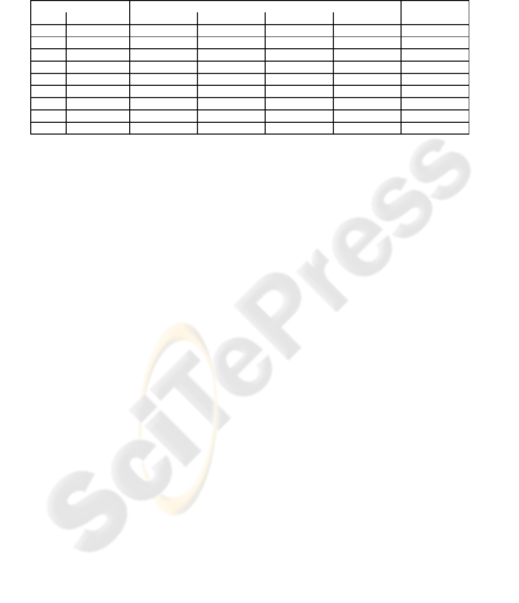
Table 2: Means and standard deviations (%) of true positive rates (TPR), positive predictive values (PPV) and total classifica-
tion accuracies (ACC) for the three best architectures of each tested neural network classifier type. The best architecture for
each classifier type is in bold.
Classifier TPR PPV ACC
Type Architecture Healthy Patient Healthy Patient
MLP 6-1 95.7 (± 15.6) 86.4 (± 22.9) 88.2 (± 19.8) 94.2 (± 17.8) 91.2 (± 13.1)
MLP 5-1 94.8 (± 18.2) 87.7 (± 21.4) 88.2 (± 21.1) 95.0 (± 15.5) 91.4 (± 13.6)
MLP 1 97.5 (± 5.3) 88.9 (± 20.3) 92.0 (± 13.0) 96.6 (± 10.0) 93.3 (± 9.7)
PNN 0.03 99.5 (± 1.8) 81.8 (± 23.8) 87.1 (± 16.0) 99.2 (± 3.8) 90.6 (± 11.9)
PNN 0.02 99.2 (± 2.6) 82.7 (± 23.2) 87.7 (± 15.8) 99.1 (± 2.8) 90.9 (± 11.6)
PNN 0.01 99.2 (± 2.1) 84.4 (± 21.9) 88.8 (± 14.7) 98.9 (± 4.9) 91.8 (± 10.8)
SOM 1 × 7 94.9 (± 7.5) 86.1 (± 19.8) 89.4 (± 14.3) 94.9 (± 6.9) 90.5 (± 9.9)
SOM 1 × 4 95.4 (± 7.3) 86.1 (± 19.9) 89.5 (± 14.3) 95.4 (± 6.4) 90.8 (± 9.9)
SOM 1 × 6 99.5 (± 1.6) 82.2 (± 24.2) 87.6 (± 15.8) 98.6 (± 9.5) 90.9 (± 11.9)
and SOM and almost 10 % with MLP. The difficulty
of recognizing the patient class is reflected also with
the standard deviations of the TPRs of the patient
class which were considerably higher than those of
the healthy class.
The PPVs show that the most of the misclassifica-
tions for all classifier types occurred when a patient
was classified into the healthy class. Indeed, the re-
sults show that confidence for the correct decision is
high for all classifiers when they decided that a sam-
ple belongs to the patient class. For the best MLP
classifier the PPVs of the both classes were well over
90 % and the difference between the two classes was
only 4.6 %. Again, for PNN and SOM the PPVs for
the patient class were extremely high, but the overall
performance was deteriorated with significantly lower
PPV values for the healthy class. The differences be-
tween PPVs of the classes were over 10 % for the best
PNN and SOM classifiers.
Based on the Friedman test results, MLP and PNN
performed statistically equally well. However, the
differences between the classification accuracies of
MLP and SOM and PNN and SOM were statistically
significant with SOM being statistically an inferior
classifier than the others. These results were statis-
tically highly significant (at level α = 0.001).
For MLP, the best performing architecture was a
network with only one node. It generally had clas-
sification accuracy almost 2 % higher than the other
tested architectures. PNN performed the best with
Gaussian window width of 0.01. Generally, increas-
ing the window width deteriorated the performance
of the network and the difference between the accu-
racies of a network with the best performing window
width 0.01 and the worst performing window width
0.06 was ca 2 %. For SOM, the best performing lat-
tice structure was 1 × 6. Other tested lattice structures
performed slightly worse their classification accura-
cies being 1 – 2 % lower than the best performing 1
× 6 lattice structure.
4 CONCLUSIONS
The results show clearly that MLP performed best in
separating the aphasic speakers from healthy speak-
ers based on their naming data distributions. MLP’s
total classification accuracy was 1 – 2 % higher than
the accuracies of the other classifier types, and their
smaller standard deviations of the classification ac-
curacies proved it also to be a more robust classifier
than the other tested classifiers. Furthermore, because
only one node was needed to implement the most
successful MLP architecture, other simple classifica-
tion methods, such as discriminant analysis and Bayes
classifiers should also perform well at the classifica-
tion task.
Based on the TPRs and PPVs all classifiers were
biased towards the healthy class. The MLP archi-
tecture favors least healthy data over patient data re-
sulting into highest overall classification accuracy of
the compared classifiers. The other two classifiers
were even more biased towards the healthy class and
correspondingly their classification accuracies were
slightly lower than MLP classifiers. The SOM clas-
sifier was clearly the weakest classifier type and the
differences of the classification accuracies to the other
two classifiers were statistically significant. Based on
these results, SOM classifiers should not be preferred
in patient / healthy classification over simpler classi-
fication methods.
The differences between the average classification
accuracies of the classifiers were very small and all
classifiers had total classification accuracy over 90 %.
Therefore, it seems that the choice of classification

method is not very crucial for the reported data set.
This also supports the choice of the simplest classi-
fier type, the one node MLP, as a preferred classifier.
However, it has to be noted that the classification task
might have been harder if more real data had been
available serving as a basis for the data generation.
On the other hand, the results with the current data
suggest that neurolinguistic tests used in aphasia test-
ing separate quite well the healthy subjects and pa-
tients from each other. Thus, it is possible that there is
no need for using more advanced classification meth-
ods in patient / healthy subject separation.
The current classification research should be ex-
tended to include more classifier types. Especially
traditional classifiers types, such as na¨ıve Bayes clas-
sifier, discriminant analysis or k-nearest neighbor
classifiers should be investigated, since the success of
the one neuron MLP classifiers suggest that the sim-
ple classification methods might perform noticeably
well with the classification task.
An important question is also how well the used
data generation method preserves the characteristics
of the original data. This question should be exam-
ined in more detail in order to ensure that the data gen-
eration does not unnaturally bias the data. Moreover,
other aphasia data sets should be tested, althoughfind-
ing a suitable data set with decent number of test cases
seems to be problematic.
ACKNOWLEDGEMENTS
The author gratefully acknowledges Professor Martti
Juhola, Ph.D., from Department of Computer Sci-
ences, University of Tampere, Finland for his help-
ful comments on the draft of the paper and Tampere
Graduate School in Information Science and Engi-
neering (TISE) for financial support.
REFERENCES
Axer, H., Jantzen, J., and von Keyserlingk, D. G. (2000).
An aphasia database on the Internet: a model for
computer-assisted analysis in aphasiology. Brain and
Language, 75(3):390–398.
Connover, W. J. (1999). Practical Nonparametric Statistics.
John Wiley & Sons, New York, NY, USA, 3 edition.
Cuetos, F., Aguado, G., Izura, C., and Ellis, A. W. (2002).
Aphasic naming in spanish: predictors and errors.
Brain and Language, 82(3):344–365.
Dell, G. S., Schwartz, M. F., Martin, N., Saffran, E. M.,
and Gagnon, D. A. (1997). Lexical access in apha-
sic and nonaphasic speakers. Psychological Review,
104(4):801–838.
Duda, R. O., Hart, P. E., and Stork, D. G. (2001). Pattern
Classification. John Wiley & Sons, New York, NY,
USA, 2 edition.
Goodglass, H. and Kaplan, E. (1983). The Assessment
of Aphasia and Related Disorders. Lea & Febiger,
Philadelphia, PA, USA, 2 edition.
Harley, T. (2001). The Psychology of Language. Psychol-
ogy Press, New York, NY, USA, 2 edition.
Haykin, S. (1999). Neural Networks. A Comprehensive
Foundation. Prentice Hall, London, United Kingdom,
2 edition.
Huber, W., Poeck, K., and Weniger, D. (1984). The Aachen
aphasia test. In Rose, F. C., editor, Advances in Neu-
rology. Progress in Aphasiology, volume 42, pages
291–303. Raven, New York, NY, USA.
Kohonen, T. (1998). The self-organizing map. Neurocom-
puting, 21(1–3):1–6.
Kohonen, T. (2001). Self-Organizing Maps. Springer-
Verlag, Berlin, Germany, 3 edition.
Laine, M., Kujala, P., Niemi, J., and Uusipaikka, E. (1992).
On the nature of naming difficulties in aphasia. Cor-
tex, 28:537–554.
Raymer, A. M. and Rothi, L. J. G. (2002). Clinical diag-
nosis and treatment of naming disorders. In Hillis,
A. E., editor, The Handbook of Adult Language Dis-
orders, pages 163–182. Psychology Press, New York,
NY, USA.
Roach, A., Schwartz, M. F., Martin, N., Grewal, R. S., and
Brecher, A. (1996). The Philadelphia Naming Test:
Scoring and rationale. Clinical Aphasiology, 24:121–
133.
Specht, D. (1990). Probabilistic neural networks. Neural
Networks, 3(1):109–118.
