REAL
TIME TRACKING OF AN OMNIDIRECTIONAL ROBOT
An Extended Kalman Filter Approach
Jos
´
e Gonc¸alves, Jos
´
e Lima
Department of Electrical Engineering, Polytechnic Institute of Braganc¸a, Portugal
Paulo Costa
Deec, Faculty of Engineering of the University of Porto, Portugal
Keywords:
Probabilistic robotics, Kalman Filter, Omnidirectional robots.
Abstract:
This paper describes a robust localization system, similar to the used by the teams participating in the Robocup
Small size league (SLL). The system, developed in Object Pascal, allows real time localization and control
of an autonomous omnidirectional mobile robot. The localization algorithm is done resorting to odometry
and global vision data fusion, applying an extended Kalman filter, being this method a standard approach for
reducing the error in a least squares sense, using measurements from different sources.
1 INTRODUCTION
Soccer was the original motivation for Robocup. Be-
sides being a very popular sport worldwide, soccer
brings up a set of challenges for researchers while
attracting people to the event, promoting robotics
among students, researchers and general public.
RoboCup chose to use soccer game as a central topic
of research, aiming at innovations to be applied for so-
cially significant problems and industries (rob, 2008).
As robotics soccer is a challenge in an highly dy-
namic environment, the robot and ball position infor-
mation must be accessible as fast and accurate as pos-
sible (Sousa, 2003). As an example if the ball has
a velocity of 2 ms
−1
and if the lag time is 100 ms,
the ball will travel a distance of 20 cm between two
sampling instants, compromising the controller per-
formance (Gonc¸alves et al., 2007). The presented lo-
calization algorithm is updated 25 times per second,
fulfilling the proposed real time requisites.
Robots maintain a set of hypotheses with regard
to their position and the position of different ob-
jects around them. The input for updating these
beliefs come from poses belief and various sensors
(Borestein et al., 1996). An optimal estimation can be
applied in order to update their beliefs as accurately as
possible. After one action the pose belief is updated
based on data collected up to that point in time, by a
process called filtering (Thrun et al., 2005).
2 RELATIVE POSITION
ESTIMATION
Omnidirectional vehicles are widely used in robotics
soccer, allowing movements in every direction, where
the extra mobility is an important advantage. The fact
that the robot is able to move from one place to an-
other with independent linear and angular velocities
contributes to minimize the time to react, the num-
ber of maneuvers is reduced and consequently the
game strategy can be simplified (Ribeiro et al., 2004).
The omnidirectional robots use special wheels, that
allow movements in every direction. The movement
of these robots does not have the restraints of the dif-
ferential robots (Dudek and Jenkin, 2000), presenting
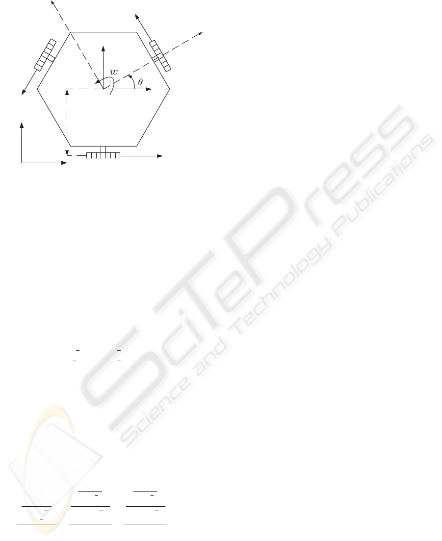
the disadvantage of a more complex control. It is pos-
sible to conclude from the geometry of a three wheel
omnidirectional robot, presented in Figure 1, that the
velocities V
x
, V
y
and w vary with the linear veloci-
ties V
1
, V
2
and V
3
, as shown in equations system (1)
(Kalm
´
ar-Nagy et al., 2002).


V
1
V
2
V
3


=


−sin(θ) cos(θ) L
−sin(
π
3
− θ) −cos(
π
3
− θ) L
sin(
π
3
+ θ) −cos(
π
3
+ θ) L




V
x
V
y
w


(1)
5
Gonçalves J., Lima J. and Costa P. (2008).
REAL TIME TRACKING OF AN OMNIDIRECTIONAL ROBOT - An Extended Kalman Filter Approach.
In Proceedings of the Fifth International Conference on Informatics in Control, Automation and Robotics - RA, pages 5-10
DOI: 10.5220/0001474500050010
Copyright
c
 SciTePress

V1
V2
V3
X
Y
L
Vx
Vy
V
Vn
Figure 1: Geometry of a three wheel omnidirectional robot.
2.1 Odometry Calculation
The robot relative position estimation is based on the
odometry calculation. The odometry calculation uses
each wheel velocity in order to estimate the robot po-
sition, the disadvantage is that the position estimate
error is cumulative and increases over time.
The robot kinematic equations can be represented
by the equations system (2), in alternative to the equa-
tions system (1).


V
1
V
2
V
3


=


0 1 L
−sin(
π
3
) −cos(
π
3
) L
sin(
π
3
) −cos(
π
3
) L




V
V
n
w


(2)
The linear and angular velocities V , V
n
and w can
be obtained rewriting equations system (2) as equa-
tions system (3),


V
V
n
w


=
¡
G
¢


V
1
V
2
V
3


(3)
where G is :




0
−1
2sin(
π
3
)
1
2sin(
π
3
)
1
1+cos(
π
3
)
−1
2(1+cos(
π
3
))
−1
2(1+cos(
π
3
))
cos
π
3
L(1+cos(
π
3
))
1
2L(1+cos(
π
3
))
1
2L(1+cos(
π
3
))




(4)
By this way θ can be found, applying an first order
approximation, as shown in equation (5),
θ(K) = θ(K − 1) + wT (5)
where T is the sampling time.
After θ calculation an rotation matrix, presented
in matrix (6), is applied in order to obtain V
x
and V
y
,
as shown in equations system (7),
B
=


cos(θ) −sin(θ) 0
sin(θ) cos(θ) 0
0 0 1


(6)


V
x
V
y
w


=
BG


V
1
V
2
V
3


(7)
x and y estimate is calculated applying an first or-
der approximation, as shown in equations (8) and (9),
x(K) = x(K − 1) +V
x
T (8)
y(K) = y(K − 1) +V
y
T (9)
where T is the Sampling Time.
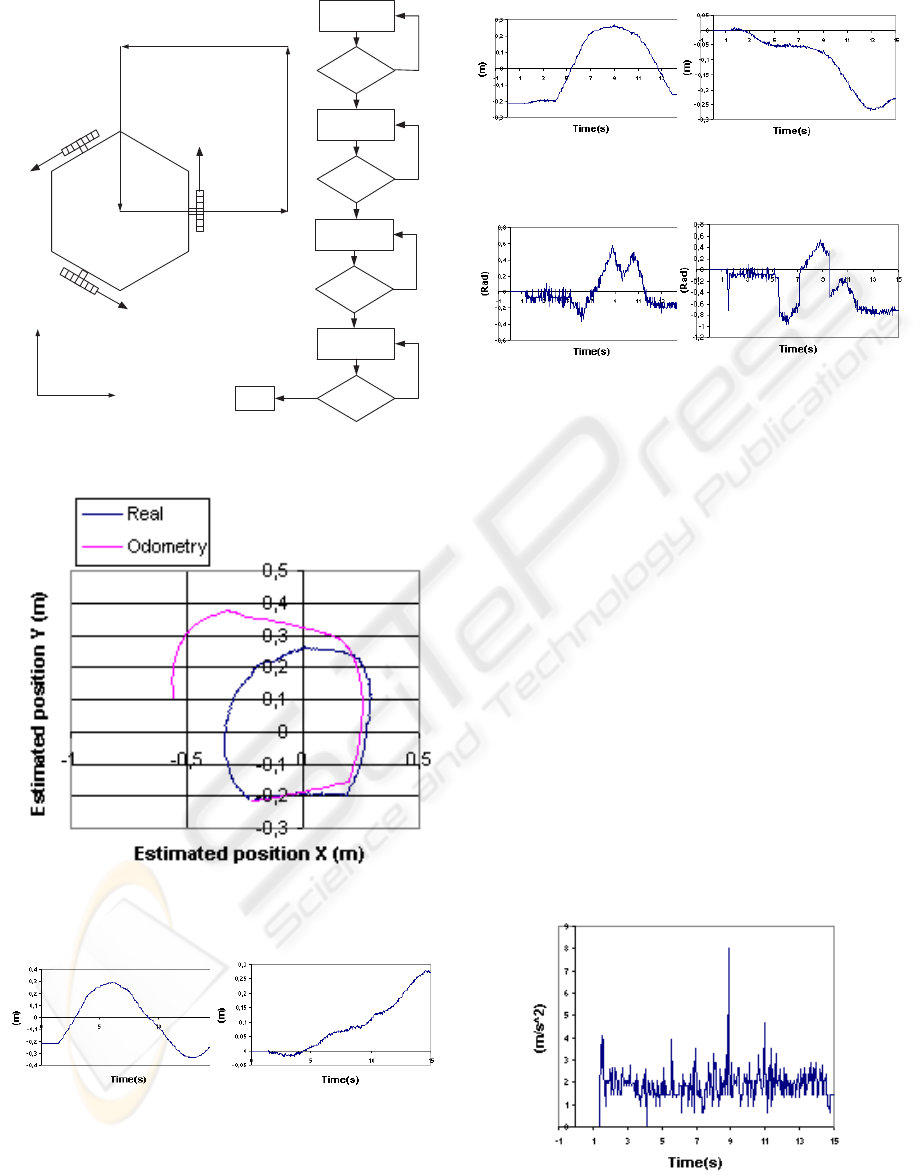
2.2 Odometry Error Study
With the objective of evaluate the odometry error a
robot race was made, as shown in the flowchart pre-
sented in Figure 2. It is possible to observe that the
robot moves across several locations, executing the
trajectory presented in Figures 3, 4, 5 and 6.
The goal of the controller is to move the robot to a
target position with controlled velocity. As input pa-
rameters we have as goal the robot displacement to
a target position. Initially a position vector pointing
to the target position is calculated, the position vec-
tor is normalized converting it into a velocity vector,
becoming this the objective to accomplish. The equa-
tions (1) are used to calculate the velocity that each
wheel must have in order to accomplish the objec-
tive. At each sampling time the estimated position
changes, consequently the position vector changes,
the velocity vector changes and the reference speed of
each motor changes. The controller has also as objec-
tive to follow the trajectory with an angle near to zero.
One important fact that needs to be enhanced from the
graphics presented in Figures 3, 4 and 5, is that when
it is expected the robot to pass by the position x = 20
cm and y = −20 cm, the robot starts to move to the
next target position. This happens because the objec-
tive of reaching one position is accomplished if the
error in x and in y is less than 2 cm, making the state
machine evolve to the next state, changing the objec-
tive to x = 20 cm and y = 20 cm.
The presented graphics (Figures 2, 4, 5, 6 and 7),
allow to obtain the odometry error model, relating
the acceleration with the odometry error. If the robot
accelerates there is an error increase because the ac-
celeration forces the wheels to slip. This situation is
ICINCO 2008 - International Conference on Informatics in Control, Automation and Robotics
6

V1
V2
V3
x=0 cm
y=0 cm
x=40 cm
y=0 cm
x=40 cm
y=40 cm
x=0 cm
y=40 cm
x
y
objective:
displacement to x=40
y=0
Objective
accomplished
Yes
No
objective:
displacement to x=40
y=40
Objective
accomplished
Yes
No
objective:
displacement to x=0
y=40
Objective
accomplished
Yes
No
End
objective:
displacement to x=0
x=0
Objective
accomplished
No
Yes
Figure 2: Flowchart of the robot race.
Figure 3: Estimated and real robot trajectory.
Figure 4: a) Real position x, and (b) Odometry x error.
more observable when the robot trajectory changes its
direction, causing the robot to decelerate and to accel-
erate causing disturbances in the robot angle, increas-
ing the angle error and consequently changing the rate
Figure 5: a) Real position y, and (b) Odometry y error.
Figure 6: a) Real angle, and (b) Odometry angle error.
that the estimate position error evolves.
By this way, if the robot is not moving the vari-
ance for x and y is considered null and if the robot is
moving the used odometry variance error model for x
and y is:
Var
xy
= K
1
+ K
2
la(k − 1)
2
(10)
• K
1
is the variance when the robot is moving in
steady state.
• K
2
is a constant that relates the variance with the
previous sample time acceleration la(k − 1).
The previous sample time acceleration is used in-
stead of the present sample time because it is more
representative to evaluate the odometry error noise,
because the encoder transitions (necessary to calcu-
late each well velocity estimation resorting to an first
order approximation) are updated from the previous
sample time up to the present sample time. The angle
variance is modeled in a similar way.
Figure 7: Linear acceleration modulus.
REAL TIME TRACKING OF AN OMNIDIRECTIONAL ROBOT - An Extended Kalman Filter Approach
7

3 ABSOLUTE POSITION
ESTIMATION
The Global vision system is required to detect and
track a mobile robot in an area supervised by one
camera. The camera is placed perpendicular to the
ground, fixed to an metallic structure, allowing a max-
imal height of 3 meters, although in the presented case
is placed only at 2 meters height. Placing the camera
higher reduces the parallax error, reduces problems
such as ball occlusion and the vision field increases,
although the image quality decreases and the error
due to the barrel distortion effect increases. The im-
age quality concept, in this case study, is related with
the number of pixels that are available at each frame
to identify and localize an robot marker. The markers,
placed on the robot top, have the goal to provide infor-
mation about the robot localization. Their geometric
shape is a circle, all with the same dimensions and
with different colors. The number of observed pixels
for each marker depends on the illumination condi-
tions, color calibration and camera height. If the cam-
era is placed higher the vision field is bigger, conse-
quently the maximum number of observed pixels for
each marker will be reduced.
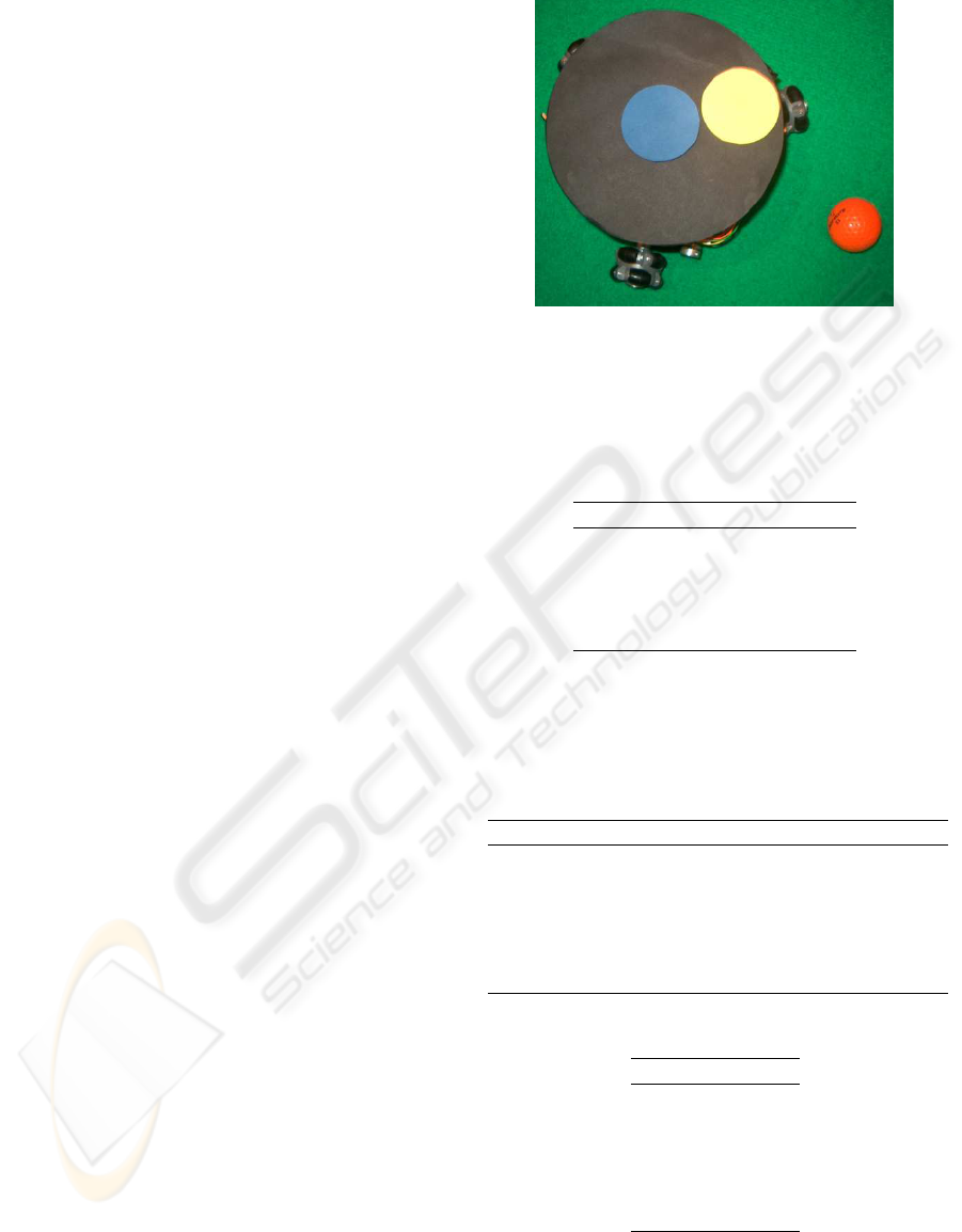
3.1 Robot Localization
Knowing at first hand that are necessary to localize
the robot two different markers, one to identify the
center and another to provide information for the an-
gle calculation. Being the field green, and the ball
orange, the colors for the robot markers should be the
most distant as possible in the RGB cube. The chosen
colors were blue for the robot center and yellow for
the angle, being the official Robocup colors to distin-
guish two teams in the SSL placing a colored marker
in each robot center (rob, 2008). The ball localiza-
tion is achieved the same way as the robot center, the
only difference is that is a marker placed at a different
height and associated to a different color. The blue
and yellow markers are used for the robot detection
and localization. The blue marker allows x and y cal-
culation, and the yellow marker allows the angle cal-
culation. The used robot is illustrated in Figure 8.
3.2 Global Vision Error Study
It was made for the global vision localization sys-
tem an analysis of the error probability distributions
(Thrun et al., 2005)(Choset et al., 2005). The posi-
tion error probability distributions were approximated
to Gaussian distributions (Ribeiro, 2004)(Negenborn,
2003), being the results presented in SI units. The
Figure 8: Omnidirectional robot prototype.
number of obtained pixels for the blue marker (Q1),
affects the error variance in x and y, as shown in the
next table:
Table 1.
Q1 x y
5-10 1,5E-05 1,9E-05
10-20 9,25E-06 7,36E-06
20-30 4,84E-06 4,86E-06
30-40 4,15E-06 3,80E-06
≥ 40 1,96E-06 2,21E-06
On the other hand the variance of the angle error
probability distribution is affected by the number of
pixels obtained for both makers, for the blue (Q1) and
for the yellow (Q2), as shown in the next tables:
Table 2.
Q1 5-10 10-20 20-30 30-40
5-10 0,14 8E-02 1,2E-02 1E-02
10-20 1,6E-02 9,9E-03 1,3E-02 6,6E-03
20-30 1,5E-02 9,9E-03 7,2E-03 4,9E-03
30-40 1,4E-02 9,5E-03 5,9E-03 4,4E-03
≥ 40 1,4E-02 7,2E-03 5,77E-03 3E-03
Q2
Table 3.
Q1 ≥ 40
5-10 6,2E-03
10-20 4,6E-03
20-30 3,9E-03
30-40 2,9E-03
≥ 40 3E-03
Q2
ICINCO 2008 - International Conference on Informatics in Control, Automation and Robotics
8

4 ODOMETRY AND GLOBAL
VISION DATA FUSION
Odometry and global vision data fusion was achieved
applying an extended Kalman filter. This method was
chosen because the robot motion equations are non-
linear and also because the measurements error prob-
ability distributions can be approximated to Gaussian
distributions (Choset et al., 2005).
4.1 Extended Kalman Filter Algorithm
With the dynamic model given by equations system
(7) and considering that control signals change only
at sampling instants, the state equation is:
dX(t)
dt
= f (X(t), u(t
k
), t), tε[t
k
, t
k+1
] (11)
Where u(t) = [V
1
V
2
V
3
]
T
, that is, the odometry
measurements are used as kinematic model inputs.
This state should be linearized over t = t
k
, X (t) =
X(t
k
) and u(t) = u(t
k
), resulting in:
A
∗
k
=



0 0
−sin(θ)
2sin(
π
3
)
+
cos(θ)
2(1+cos(
π
3
))
0 0
cos(θ)
2sin(
π
3
)
+
sin(θ)
2(1+cos(
π
3
))
0 0 0



(12)
with state transition matrix:
φ
∗
(k) = exp(A
∗
(k)(t
k
−t
k−1
)) (13)
Resulting in:
φ
∗
k
=



1 0 (
−sin(θ)
2sin(
π
3
)
+
cos(θ)
2(1+cos(
π
3
))
)T
0 1 (
cos(θ)
2sin(
π
3
)
+
sin(θ)
2(1+cos(
π
3
))
)T
0 0 1



(14)
Where T is the sampling time (t
k
−t
k−1
).
Thus the observations are obtained directly, H
∗
is
the identity matrix.
The extended Kalman filter algorithm steps are as
follows (Welch and Bishop, 2001):
1. State estimation at time t = t
k
, X(k
−
), knowing the
previous estimate at t = t
k−1
, X(k − 1) and con-
trol u(t
k
), calculated by numerical integration as
shown in equations (5), (8) and (9).
2. Propagation of the state covariance
P(k
−
) = φ
∗
(k)P(k − 1)φ
∗
(k)
T
+ Q(k) (15)
Where Q(k) is the noise covariance (11) and also
relates to the model accuracy. In order to achieve a
more realistic model of the odometry error prob-
ability distribution it is necessary to have in ac-
count that for abrupt acceleration or deceleration
the wheels can slip, consequently there is an sig-
nificant position estimate error increase, mainly in
the angle (Gonc¸alves et al., 2005).
As there is a measure, the follow also apply:
3. Kalman gain calculation
K(k) = P(k
−
)H
∗
(k)
T
(H
∗
(k)P(k
−
)H
∗
(k)
T
+ R(k))
−1
(16)
Where R(k) is the covariance matrix of the mea-
surements.
4. State covariation update
P(k) = (I − K(k)H
∗
(k))P(k
−
) (17)
5. State update
X(k) = X(k
−
) +K(k)(z(k) − h(X(k
−
, 0))) (18)
Where z(k) is the measurement vector and
h(X(k
−
, 0)) is X(k
−
).
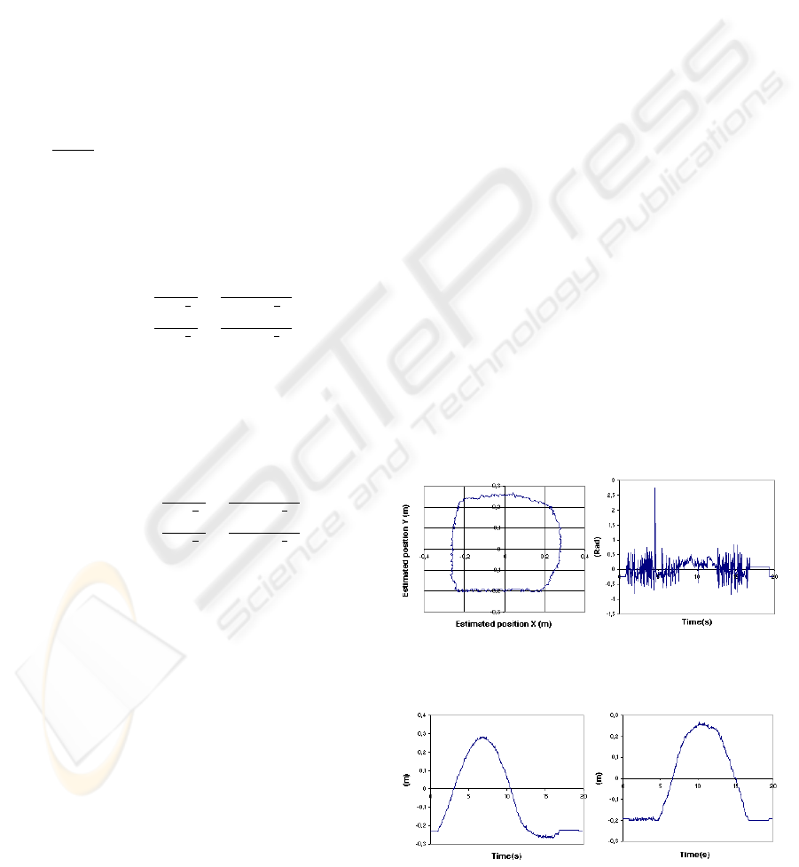
4.2 Kalman Filter Performance
With the objective of evaluating the Kalman filter per-
formance another robot race was made, as shown in
the flowchart presented in Figure 2. The robot trajec-
tory is presented in Figures 9 and 10.
Figure 9: a) Robot trajectory, and (b) Estimated Angle.
Figure 10: a)Estimated x, and (b) Estimated y.
REAL TIME TRACKING OF AN OMNIDIRECTIONAL ROBOT - An Extended Kalman Filter Approach
9

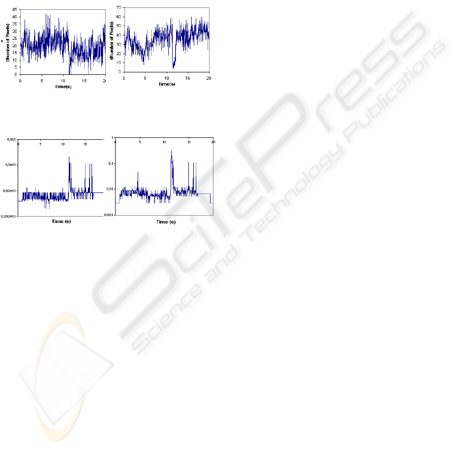
The image quality of the robot markers for the pre-
sented robot race are presented in Figure 11 and the
variance of the estimated robot position is presented
in Figure 12. Whenever the image quality decreases
the variance error of position estimate increases com-
promising the controller performance. On the other
hand whenever the image quality increases the error
variance is reduced and when the state update is done
the position estimate error is reduced.
Figure 11: a) Image quality of the center marker Q1,
b)Image quality of the angle marker Q2.
Figure 12: a) x and y variance, and (b) Angle variance.
5 CONCLUSIONS
Omnidirectional vehicles have many advantages in
robotics soccer applications, allowing movements in
every direction. The fact that the robot is able to move
from one place to another with independent linear and
angular velocities contributes to minimize the time to
react, the number of maneuvers is reduced and conse-
quently the game strategy can be simplified.
The robot relative position estimation is based on
the odometry calculation. The odometry calculation
uses each wheel velocity in order to estimate the robot
position, the disadvantage is that the position estimate
error is cumulative and increases over time.
It was made for the global vision localization sys-
tem an analysis of the error probability distributions.
The number of obtained pixels for the blue marker
(Q1), affects the error variance in x and y. On the
other hand the variance of the angle error probability
distribution is affected by the number of pixels ob-
tained for both makers, for the blue (Q1) and for the
yellow (Q2).
Odometry and global vision real time data fu-
sion was achieved applying an extended Kalman fil-
ter. This method was chosen because the robot motion
equations are nonlinear and also because the measure-
ments error probability distributions can be approxi-
mated to Gaussian distributions.
REFERENCES
(2008). Robocup. http://www.robocup.org/.
Borestein, Everett, and Feng (1996). where am I, Sensores
and Methods for Mobile Robot Positioning. Prepared
by the University of Michigan.
Choset, H., Lynch, K., Hutchinson, S., Kantor, G., Burgard,
W., Kavraki, L., and Thrun, S. (2005). Principles of
Robot Motion : Theory, Algorithms, and Implementa-
tions. MIT Press.
Dudek, G. and Jenkin, M. (2000). Computational Princi-
ples of Mobile Robotics. Cambridge University Press.
Gonc¸alves, J., Costa, P., and Moreira, A. (2005). Controlo
e estimac¸
˜
ao do posicionamento absoluto de um robot
omnidireccional de tr
ˆ
es rodas. Revista Rob
´
otica, Nr
60, pp 18-24.
Gonc¸alves, J., Pinheiro, P., Lima, J., and Costa, P. (2007).
Tutorial introdut
´
orio para as competic¸
˜
oes de futebol
rob
´
otico. IEEE RITA - Latin American Learning Tech-
nologies Journal, 2(2):63–72.
Kalm
´
ar-Nagy, T., D’Andrea, R., and Ganguly, P. (2002).
Near-optimal dynamic trajectory generation and con-
trol of an omnidirectional vehicle. In Sibley School of
Mechanical and Aerospace Engineering.
Negenborn, R. (2003). Robot Localization and Kalman Fil-
ters - On finding your position in a noisy world. Mas-
ter Thesis, Utrecht University.
Ribeiro, F., Moutinho, I., Silva, P., Fraga, C., and Pereira,
N. (2004). Controlling omni-directional wheels of a
robocup msl autonomous mobile robot. In Proceed-
ings of the Scientific Meeting of the Robotics Por-
tuguese Open.
Ribeiro, M. I. (2004). Gaussian Probability Density Func-
tions: Properties and Error Characterization. Tech-
nical Report, IST.
Sousa, A. (2003). Arquitecturas de Sistemas Rob
´
oticos e
Localizac¸
˜
ao em Tempo Real Atrav
´
es de Vis
˜
ao. PHD
Thesis, Faculty of Engineering of the University of
Porto.
Thrun, S., Burgard, W., and Fox, D. (2005). Probabilistic
robotics. MIT Press.
Welch, G. and Bishop, G. (2001). An introduction to the
Kalman filter. Technical Report, University of North
Carolina at Chapel Hill.
ICINCO 2008 - International Conference on Informatics in Control, Automation and Robotics
10