
ADAPTIVE RESOURCES CONSUMPTION IN A DYNAMIC AND
UNCERTAIN ENVIRONMENT
An Autonomous Rover Control Technique using Progressive Processing
Simon Le Gloannec, Abdel Illah Mouaddib
GREYC UMR 6072, Universit´e de Caen Basse-Normandie, Campus Cˆote de Nacre
bd Mar´echal Juin, BP5186, 14032 Caen Cedex, France
Franc¸ois Charpillet
MAIA team, LORIA, Campus Scientifique, BP 239, 54506 Vandœuvre-l`es-Nancy Cedex, France
Keywords:
MDP, Resource-bounded Reasoning, Hierarchical control, Autonomous agents, Planning and Scheduling.
Abstract:
This paper address the problem of an autonomous rover that have limited consumable resources to accomplish
a mission. The robot has to cope with limited resources: it must decide the resource among to spent at each
mission step. The resource consumption is also uncertain. Progressive processing is a meta level reasoning
model particulary adapted for this kind of mission. Previous works have shown how to obtain an optimal
resource consumption policy using a Markov decision process (MDP). Here, we make the assumption that
the mission can dynamically change during execution time. Therefore, the agent must adapt to the current
situation, in order to save resources for the most interesting future tasks. Because of the dynamic environment,
the agent cannot calculate a new optimal policy online. However, it is possible to compute an approximate
value function. We will show that the robot will behave as good as if it knew the optimal policy.
1 INTRODUCTION
Resources consumption control is crucial in the au-
tonomous rover context. For example, a rover must
know when it has to go back to a docking station be-
fore having no energy left. The question for the agent
is to know where, when, and the amount of resources
it has to spend for a particular task. We want this
agent to be adaptive : it has to choose the amount
of resources to spend in each task by taking into ac-
count the expected value. This is the reason why we
use progressive processing to modeland to control the
mission. This model of reasoning describes tasks that
can be performed progressively, with several options
at each step. The resources consumption is proba-
bilistic. Progressive processing provides a meta-level
resources consumption model. Then, we obtain an
optimal policy control thanks to a MDP.
For now, progressive processing does not cope
with dynamic environments. In a real robot applica-
tion, it is not uncommon to see new tasks incoming
during the mission. When it happens, the agent has
to completely recalculate the resource control policy
to behave optimally. Most of the time, it doesn’t have
sufficient time to do it. For these reasons, we propose
here a value function approximation method that al-
lows the agent to compute a local near optimal pol-
icy very quickly in order to cope with the dynamic
changes. We will bring experimental result to vali-
date this method.
The paper is divided into five main sections. The
third section introduces progressive processing and its
use for an autonomous rover mission application. In
the fourth section, we present the dynamic environ-
ment and propose a way to cope with changes during
the mission. This theory is experimentally validated
in the last section.
2 RELATED WORK
• Control of Progressive Processing: Progressive
processing has been introduced in (Mouaddib and
Zilberstein, 1998), and has been used in a real
rover application (Zilberstein et al., 2002) and in
a retrieval information engine (Arnt et al., 2004).
Concerningthe retrievalinformation engine, users
send requests to a server that can respond very
200
Le Gloannec S., Illah Mouaddib A. and Charpillet F. (2008).
ADAPTIVE RESOURCES CONSUMPTION IN A DYNAMIC AND UNCERTAIN ENVIRONMENT - An Autonomous Rover Control Technique using
Progressive Processing.
In Proceedings of the Fifth International Conference on Informatics in Control, Automation and Robotics - ICSO, pages 200-206
DOI: 10.5220/0001492802000206
Copyright
c
SciTePress

precisely and use lots of resources, or approxima-
tively and use less resources. Progressive process-
ing permits to model the server tasks. It also per-
mits to adapt the resources dedicated to each task
by taking the number of requests into account. We
will briefly presentthe rover application in this pa-
per.
• MDP Decomposition: an MDP is used to for-
malise the mission resource consumption control.
We can either compute an optimal policy or an
approximate policy. Our approximation is based
on MDP decomposition. This technique has been
largely studied in the literature. Dean et al (Dean
and Lin, 1995) investigated methods that decom-
pose global planning problems into a number of
local problem. In (Parr, 1998), the method is to
build a cache of policies for each part of the prob-
lem independently, and then to combinethe pieces
in separate steps. (Meuleau et al., 1998) also
proposed a decomposition technique for a prob-
lem where tasks have indepedent utilities, and are
weakly coupled.
• Value Function Approximation: our work also
deals with value functionapproximation. In (Feng
et al., 2004), the state space is dynamically par-
titioned into regions where the value function is
the same throughout the region. Authors make
piecewise constant and piecewise linear approx-
imations. (Pineau et al., 2003) introduced point
base value iteration. It approximates an exact
value iteration solution by selecting a small set
of representative belief points and by tracking the
value and its derivative for those points only.
3 MODEL A MISSION WITH
PROGRESSIVE PROCESSING
The problem formalism will be presented hierarchi-
cally: the mission is divided into progressive process-
ing units (PRU), which are separated into levels.
3.1 Formalism
A mission is a set of tasks, and each task is an acyclic
graph vertex (see Figure 1). To facilitate access to
the formalism, we assume that this acyclic graph is an
ordered sequence. This involves no loss of generality.
You can see this sequence as a particular path in the
graph (for example A, B, E, F). There are P tasks in
the sequence. Each task is modelled by a progressive
processing unit (PRU). It is structured hierarchically.
Each PRU
p
, p ∈ {1,... ,P} is a level ordered finite
sequence [L
p,1
,.. . ,L
p,L
]. An agent can process a level
only if the precedinglevel is finished. The process can
be interrupted after each level. It means that the agent
can stop the PRU execution, but it receives no reward
for it. Other situations have been proposed when the
agent can have a reward at each level. However, in our
case, only a complete task accomplishment provides
a reward.
Site
B
C
Site
E
Site
Site
D
End
F
Site
Picture analysis
Weather analysis
Rock analysis
Start
A
Site
Figure 1: A mission.
Each level L
p,ℓ
contains one or more modules
[m
p,ℓ,1
,.. . ,m
p,ℓ,M
]. A module is a specific way to ex-
ecute a level. The agent can only execute one module
per level. The execution of a module produces a qual-
ity Q and consumes resources. A progressive pro-
cessing unit definition is illustrated on Figure 2 for a
picture task. Firstly, the rover has to aim its camera,
then it chooses the picture resolution. At the end, it
saves the picture. The execution is performed from
bottom to top.
The quality Q
p,ℓ,m
∈ R
+
is a criterion to measure
the module execution impact. There is no immediate
reward after each level processing. The agent receives
the sum of all the Q
p,ℓ,m
only when the last level is
performed.
The resource consumption in a module m
p,ℓ,m
is
probabilistic. We denote as P r
p,ℓ,m
the probability dis-
tribution of resources consumption.
PRU
p
Level 1
Level 2
Level 3
4 53
R
Pr
R
2
1
0.1
0.2
0
1
2
3
4 53
R
Pr
R
2
1
0.1
0.2
0
1
2
3
4 53
R
Pr
R
2
1
0.1
0.2
0
1
2
3
4 53
R
Pr
R
2
1
0.1
0.2
0
1
2
3
4 53
R
Pr
R
2
1
0.1
0.2
0
1
2
3
4 53
R
Pr
R
2
1
0.1
0.2
0
1
2
3
4 53
R
Pr
R
2
1
0.1
0.2
0
1
2
3
ressources consumption
probability distribution
Q Q
Q
Q
Q
module quality
Q
res
med
res
high
high comp low comp
aim camera
low
res
Figure 2: PRU.
ADAPTIVE RESOURCES CONSUMPTION IN A DYNAMIC AND UNCERTAIN ENVIRONMENT - An Autonomous
Rover Control Technique using Progressive Processing
201

3.2 Mission Control
The problem of control we address in this paper con-
sists of a robot exploring an area where it has sites
to visit and performs exploration tasks. The problem
is that the robot cannot know in advance its resource
consumption. We use then a MDP to control the mis-
sion. The agent is supposed to be rational. It must
maximise the mathematical expected value. It com-
putes a policy that correspond to this criterion before
executing the mission. The on-line mission control
process consists in following this policy. In the next
section, we present the MDP model and the control
policy calculation. At each site the agent must take a
decision to stay for continuing the exploration or to
move to another site.
3.2.1 Modelling the Mission as an Markov
Decision Process
Formally, a MDP is tuple {S ,A ,P r,R } where :
• S is a finite set of states,
• A is a finite set of actions,
• P r is a mapping S × A × S → [0,1],
• R : S → R is a reward function.
Given a particular rational criterion, algorithms
for solving MDPs can return a policy π, that maps
from S to A , and a real-valued function V : S → R.
Here, the criterion is to maximise the expected reward
sum.
3.2.2 States
In the progressive processing model, a state is a tu-
ple hr,Q,p,ℓi. r is a reel number that indicates the
amount of remaining resources. Q is the cumulated
quality since the beginning of the current PRU. p and
ℓ indicates the last executed level L
p,ℓ
done. The fail-
ure state, denoted as s
failure
is reached when the re-
source quantity is negative. The reward is assigned
to the agent only when the last level of the PRU has
been successfully executed. Then, it is necessary to
store the cumulated quality Q in the state description.
We have introduced level 0 in order to represent the
situation where the agent begins the PRU execution.
3.2.3 Actions
There are two kinds of actions in the progressive
processing model. An agent can execute only one
module in the next level or move to the next PRU.
These two actions are depicted in Figure 3. Formally,
A = {E
m
,M}. When the agent reaches the last level
in a PRU
p
, it directly moves to the next PRU
p+1
.
m
2, 1
m
2, 2
m
2, 3
m
3, 2
m
3, 1
m
1, 1
E
2
E
1
M
s
next PRU
Level 1
Level 2
Level 3
Level 1
Level 3
Level 2
current PRU
m
1, 1
Figure 3: Actions.
Actually, E
m
is an improvement of the the current
PRU whereas M is an interruption. The agent can pro-
gressively improvethe PRU execution, it can also stop
it at any moment.
3.2.4 Transitions
M is a deterministic action whereas E
m
is not. Indeed,
the module execution consumes resources and this
consumption is probabilistic. After executing a given
module, the agent always cumulates a fixed quality.
The uncertainty is related to the resources consump-
tion probability distribution. Thus,
P r(hr,Q, p,ℓi,M,hr,0, p + 1,0i) = 1
P r(hr,p, Q,ℓi,E
m
,hr
′
,Q
′
,p,ℓ + 1i)= P r(∆r|m
p,ℓ,m
)
where Q
′
= Q+ Q
p,ℓ,m
and r
′
= r − ∆r
(1)
3.2.5 Reward
A reward is given to the agent as soon as it finishes a
PRU. This reward corresponds to the cumulated qual-
ity through the modules path. If the agent leaves a
PRU without finishing it, it receives no reward. This
makes a sense for explorationtask where the robothas
no reward if the task is not completely finished.
R (hr,Q,p,L
p
i) = Q (2)
R (hr,Q,p,ℓ < L
p
i) = 0 (3)
where L
p
is the number of levels in PRU
p
.
ICINCO 2008 - International Conference on Informatics in Control, Automation and Robotics
202

3.2.6 Value Function
The controlpolicy π : S → A dependson a value func-
tion that is calculated thanks to the Bellman equa-
tion 4. We assume that V (s
failure
) = 0.
V (hr,Q,p,ℓi) =
0 if r < 0 (failure)
R (hr,Q,p, ℓi) + max(V
M
,V
E
) otherwise
V
M
(hr,Q, p,ℓi) =
0 if p = P
V (hr,0,p + 1,0i) otherwise
V
E
(hr,Q, p,ℓi) =
0 if ℓ = L
p
max
E
m
∑
∆r
P r(∆r|m
p,ℓ,m
).V (hr
′
,Q
′
,p,ℓ + 1i)
where Q
′
= Q+ Q
p,ℓ,m
and r
′
= r − ∆r
(4)
Action E consumes some resources whereas M
does not. The agentwill execute the module that gives
it the best expected value.
3.3 Control Policy
The main objective is to compute a policy that the
robot will follow in order to optimise the resource
consumption during the mission. It has been proven
that we could calculate an optimal policy (Mouaddib
and Zilberstein, 1998). When the mission is fixed
before execution time, we can get this policy with a
backward chaining algorithm. With this policy, the
robot can choose at any moment the decision that
maximise the global utility function for the mission
i.e. the obtained reward sum. But, this policy is fixed
for a given mission. If the mission changes during
execution time, this policy is no longer up to date.
Even if the policy algorithm is linear in the state
space, the time needed to compute the optimal policy
is often more than a module execution time. This oc-
curs especially when the mission (and then the state
space) is large. This is the reason why we propose an
other way to calculate the policy. We will not cal-
culate an optimal policy, but a near-optimal policy
which could be used to take good decision when the
mission changes.
4 THE DYNAMIC
ENVIRONMENT
We suppose in this paper that tasks can come or dis-
appear during execution time. This assumption is re-
alistic for an explorer rover.
Instead of seeing the control as a global policy for
the mission, we decompose it in two parts, the current
PRU and the rest of the mission. The policy is only
calculated for the current PRU. It only dependson the
expected value function for the rest of the mission.
We could yet obtain the optimal policy with this
method by simply calculating the expected value
function for the rest of the mission without any ap-
proximation. Thus, we will naturally not save time.
Then, we present here a method to calculate the ex-
pected value function very quickly.
5 VALUE FUNCTION
APPROXIMATION
The quick value function approximation is based on a
decomposition technique. Decomposition techniques
are often use in large Markov decision processes.
Here, we will re-compose an approximate expected
value function in two times. Firstly, we calculate an
optimal local value function for each PRU in the mis-
sion. These local functions are splitted into function
pieces. Secondly, we re-compose the value function
with all the function pieces as soon as a change occurs
at run-time. This section is divided in two parts, the
decomposition, and the recomposition. We denote as
V
∗
the optimal value function and V
∼
its approxima-
tion. The main objective of the recomposition is to fit
V
∗
as good as possible.
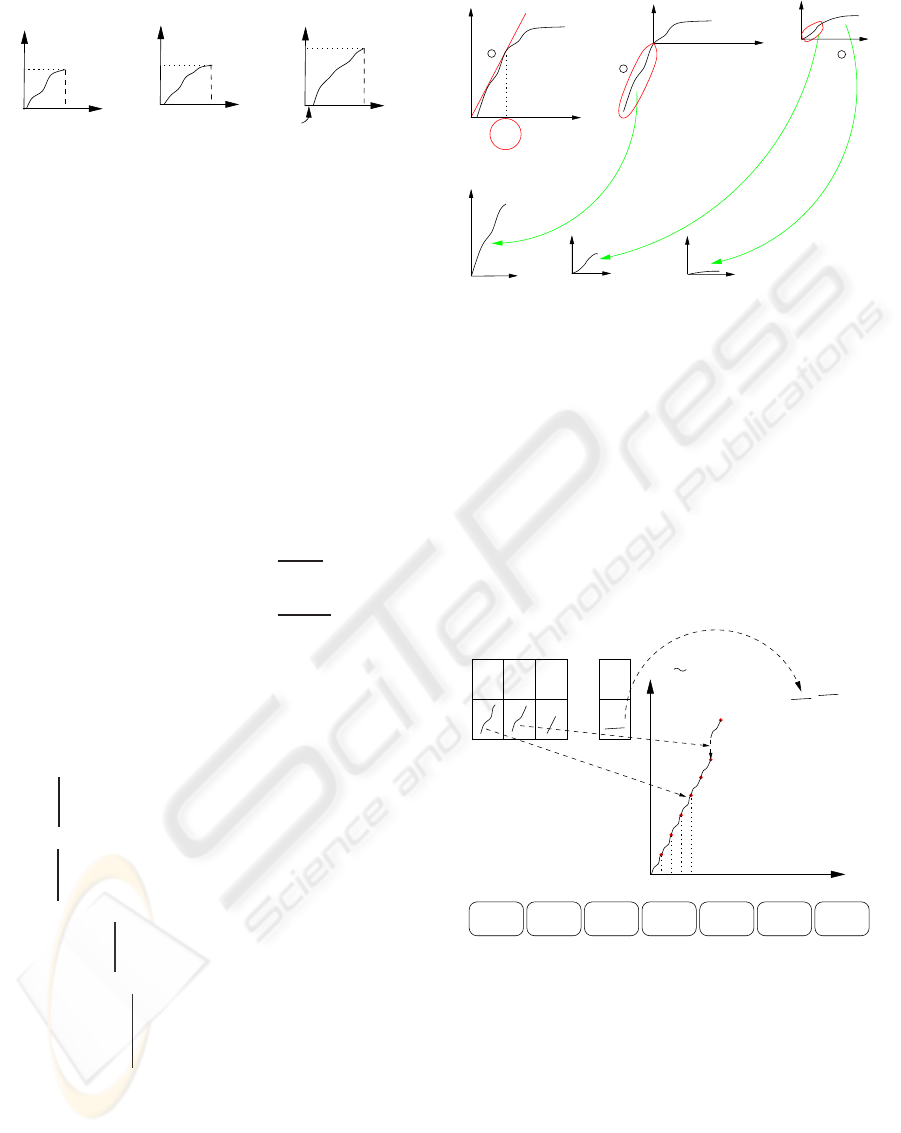
5.1 Decomposition
The decomposition consists in the calculation of the
value functions for each PRU
p
in the mission. These
functions are indeed performance profiles (denoted as
f
p
): they indicate the expected value for this PRU if
r are allocated. Three performance profiles examples
are depicted in Figure 4. The PRU γ can not consume
more than 31 resource units, and give a maximum ex-
pected value of 25.
The main idea is to use these functions to re-
compose the global approximate value function. The
performance profiles receive a preliminary treatment.
The progressive processing provides value functions
that are similar to anytime reasoning value functions :
• they increase with the allocated resource amount,
ADAPTIVE RESOURCES CONSUMPTION IN A DYNAMIC AND UNCERTAIN ENVIRONMENT - An Autonomous
Rover Control Technique using Progressive Processing
203
f (r)
α
r
max
α
R
17
20
f (r)
β
r
max
β
R
22
21
r
max
γ
f (r)
γ
R
31
25
Figure 4: 3 PRU performance profiles.
• the best improvements are made with few re-
sources, the growth of V
∗
is higher at its begin-
ning than at its end.
For these reasons we split f
p
into i
p
pieces
g
p,1
,.. . ,g
p,i
p
. During the recomposition, we will take
the best pieces to re-compose the beginning of V
∼
,
and the worst for the end. We keep the part of f
p
with the best growth, i.e. the piece between (0,0)
and (r
max
p,1
, f
p
(r
max
p,1
)). r
max
p,1
is the resource amount that
provides the best tradeoff between the resources spent
and the local expected value.
r
max
p,1
= argmax
p,r
f
p
(r)
r
(5)
∀i > 1,r
max
p,i
= argmax
p,r
f
p,i
(r)
r
(6)
When the first r
max
p,1
is found, we save the first
piece of f
p
as g
p,1
. We split f
p
in g
p,1
and f
p,2
. We
continue to search the second r
max
p,2
in f
p,2
; we save
g
p,2
etc... until f
p,i
p
is empty.
g
p,1
:
0... r
max
p,1
→ R
r → f
p
(r)
f
p,1
:
0... r
max
p
− r
max
p,1
→ R
r → f
p
(r − r
max
p,1
) − f
p
(r
max
p,1
)
∀i > 1,
g
p,i
:
0... r
max
p,i
→ R
r → f
p,i
(r)
∀i ≥ 1,
f
p,i+1
:
0... r
max
p
−
∑
i
j=1
r
max
p, j
→ R
r → f
p,i
(r − r
max
p,i
) − f
p,i
(r
max
p,i
)
(7)
Figure 5 illustrates the decomposition method for
one PRU performance profile f
p
.
All PRU are treated in the same way, such that we
obtain a list of performance profile pieces {g
p,i
,1 ≤
p ≤ P,1 ≤ i ≤ i
p
}. We sort this set with the best trade-
off criterion : g
p,i
(r
max
p,i
)/r
max
p,i
. When this set is sorted,
the agent is ready to re-composeV
∼
.
b
b
b
f (r)
p,2
f (r) =
p,2
r
r
r
p,1
r
p,1
r
r
p,1
p,1
p
p
r
p,3
g (r)
f ( − r) − f ( )
pieces
performance
profile
p
f (r)
r
p,2
g (r)
r
max
max
max
g (r)
Figure 5: Decomposition.
5.2 Recomposition
When the mission changes during execution time, the
agent re-composes V
∼
by assembling all the pieces.
The first g element is the one with the best growth,
and so on. The method is depicted on Figure 6. V
∼
and V
∗
have the same support [0... r
max
]. In order
to know the expected value for a given amount r, the
agent check the value V
∼
(r). Then, it will take its
local decision according to this approximate value.
performance profiles
pieces list (sorted)
r
r 2.r 3.r 4.r 4.r + r
1 1 1 1 1 2
...
...
V (r)
mission :
1
PRU
2
PRU
3
PRU
4
PRU
5
PRU
6
PRU
7
PRU
max max max max
r r rr
1,1 2,1 1,2 4,2
Figure 6: V
∼
recomposition.
6 VALIDATION
In the previous sections, we present how to obtain an
approximation of the value function. The rover will
use this function in order to take decision if the mis-
sion change during execution time. Now, we must
prove that :
• the time needed to obtain V
∼
is short enough,
ICINCO 2008 - International Conference on Informatics in Control, Automation and Robotics
204
• the rover can take good decisions by using V
∼
.
Concerning the time needed to calculate V
∼
, we ob-
tain very good results : it takes just few milliseconds.
Tabular 1 give computation time for different mission
sizes.
Table 1.
# PRUs 20 40 60 80 100 120 140
V
∗
(in s) 3 7 16 35 63 112 187
V
∼
(in ms) 0,4 0,9 1,2 1,7 2,2 2,6 3,5
To validate our approach, we will show that the
agent can take good decisions by using V
∼
as an ex-
pected value. The decision quality evaluation is made
throw the Q-value function comparison for each pair
(state,action) between the policies locally obtained
with V
∼
and V
∗
.
The validation consists in four steps :
1. we calculate both V
∼
and V
∗
,
2. we calculate both policies (π
∗
0
and π
∼
0
) for the cur-
rent PRU
0
,
3. we calculate Q
∗
0
, the local optimal Q-value func-
tion (for PRU
0
),
4. compare the loss of value while the agent is using
π
∼
0
instead of π
∗
0
.
Note that point 2 and 3 are done together at the same
time. As the MDP for PRU
0
has few states, the calcu-
lation of π
∗
0
, Q
∗
0
and π
∼
0
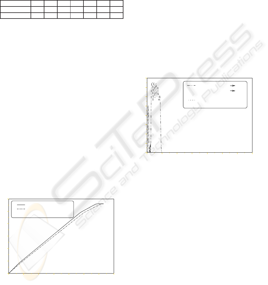
is quick. We did some experi-
ments with mission composed of different PRU kinds
and number. Figure 7 is an example of V
∼
and V
∗
for
20 PRU with 4 PRU kinds.
R
V*
V~
V
0 100 200 300 400 500 600 700
0
100
200
300
400
500
600
Figure 7: V
∼
and V
∗
.
On this Figure 7 we see that V
∼
is a good approx-
imation ofV
∗
. We have done several experiments and
have obtain some good results. Q
∗
0
is given by the
following equation.
Q
∗
0
(hr,Q,0,ℓi, E
m
) = V
E
m
(hr,Q,0,ℓi) (8)
Q
∗
0
(hr,Q,0,ℓi, M) = V
∗
(r) (9)
It makes no sense to calculate the Q-value for π
∼
0
.
When the agent takes its decisions using π
∼
0
instead
of π
∗
0
, there may be a loss of value. The error value is
given by :
e(s) = Q
∗
0
(s,π
∗
0
(s)) − Q
∗
0
(s,π
∼
0
(s)) (10)
Indeed, if for a given state s, π
∗
0
(s) = π
∼
0
(s), then the
error is zero. Otherwise, e(s) measure the loss of
value. The objective is to obtain as few error as possi-
ble. When an error exists, the better is to have a small
value.
∆ Qe =
V : R IR
0r
R
e
e
V~
0 100 200 300 400 500 600 700
0.0
0.4
0.8
1.2
1.6
2.0
2.4
2.8
3.2
Figure 8: V
∼
and V
∗
.
Figure 8 is an error measure with V
∼
and V
∗
de-
picted on Figure 7. When we use our approximation
method, there is no error. It explains why we do not
see any dotted curve on the Figure. The other curve
correspondsis the error measure if the agentconsiders
that the expected value is null (V(r) = 0). When the
robot has few resources, it does not always take an
optimal decision. However, when the agent follows
our approximative policy, it never make mistakes.
Of course, this example seems to be chosen be-
cause it is the best. But it is not the case. We made
some experiments with two different PRU kinds. The
first PRU kind is composed of tightened modules :
near qualities, near resource consumption. On the
contrary, the second PRU kind is composed of distant
modules : separate qualities, distant resource con-
sumption.
When the agent calculates π
∼
0
on a PRU of the first
type, there are lots of errors. Indeed, the modules are
almost the same, so the Q-value difference between
two actions is low. Then, it is very difficult for the
ADAPTIVE RESOURCES CONSUMPTION IN A DYNAMIC AND UNCERTAIN ENVIRONMENT - An Autonomous
Rover Control Technique using Progressive Processing
205

agent to take the right decision. However, in this case,
the error is also low. When the agent chooses a mod-
ule that is near of the optimal one, it does not make
the right decision, but this decision is good.
When the agent calculates π
∼
0
on a PRU of the sec-
ond type, there are few errors. For a given state, Q-
values are separate because the module qualities are
separate. Then, most of the time π
∼
0
is equal to π
∗
0
,
the robot chooses the right decision.
To conclude, if modules are clearly separate, the
robot takes the right decision. If modules are near,
the robot takes good decisions, with a low Q-value
error level.
6.1 Limits of this Approximation
Method
The resource consumption probability distribution
follows a normal distribution law in all the modules
we use for our experiments. Most of the time, it rep-
resents modules that can be found a real application.
We have also tried to make some experiments with
modules in which the resource consumption proba-
bility distribution is not normal. We made a risky
module m : the resource consumption is 4 or 16, with
P r(4|m) = 0.5 and P r(16|m) = 0.5. In this case the
module can only consume 4 or 16 units, but not 8.
In this kind of particular case V
∗
is not smooth. As
a result, V
∼
is not a good approximation. Then, π
∼
0
and π
∗
0
are different, there is a lot of error. But this
case does not represent a realistic resource consump-
tion module.
7 CONCLUSIONS
Resource consumption is crucial for an autonomous
rover. Here, this rover has to cope with limited re-
sources to executed a mission composed of hierarchi-
cal tasks. These tasks are progressiveprocessing units
(PRU). It is possible to compute an optimal resource
control for the entire mission by modelling it with an
MDP. In the case where the mission changes at exe-
cution time, the rover has to recompute online a new
global policy. We propose a way to quickly compute
an approximate value function that can be used to cal-
culate a local policy on the current PRU. MDP De-
composition and value function approximation tech-
niques are used to calculate V
∼
. We have shown in
the last section that the agent takes good decisions
when it uses V
∼
to compute its local policy π
∼
0
. In
a near future, we intend to complete our demonstra-
tion on real robots by considering dynamic situations
where missions can change online.
REFERENCES
Arnt, A., Zilberstein, S., Allan, J., and Mouaddib, A.
(2004). Dynamic composition of information retrieval
techniques. Journal of Intelligent Information Sys-
tems, 23(1):67–97.
Dean, T. and Lin, S. H. (1995). Decomposition techniques
for planning in stochastic domains. In proceedings
of the 14th International Joint Conference on Artifi-
cial Intelligence (IJCAI), pages 1121–1127, Montreal,
Quebec, Canada.
Feng, Z., Dearden, R., Meuleau, N., and Washington, R.
(2004). Dynamic programming for structured contin-
uous markov decision problems. In proceedings of
UAI 2004, pages 154–161.
Meuleau, N., Hauskrecht, M., Kim, K., Peshkin, L., Keal-
bling, L., Dean, T., and Boutilier, C. (1998). Solving
very large weakly coupled markov decision processes.
In proceedings of the 14th Conference on Uncertainty
in Artificial Intelligence, Madison, WI.
Mouaddib, A. I. and Zilberstein, S. (1998). Optimal
scheduling for dynamic progressive processing. In
proceedings of ECAI, pages 499–503.
Parr, R. (1998). Flexible decomposition algorithms for
weakly coupled markov decision process. In proceed-
ings of the 14th Conference on Uncertainty in Artifi-
cial Intelligence, Madison, WI.
Pineau, J., Gordon, G. J., and Thrun, S. (2003). Point-based
value iteration: An anytime algorithm for pomdps.
In proceedings of the 18th International Joint Con-
ference on Artificial Intelligence IJCAI, pages 1025–
1032.
Zilberstein, S., Washington, R., Berstein, D., and Mouad-
dib, A. (2002). Decision-theoretic control of planetary
rovers. LNAI, 2466(1):270–289.
ICINCO 2008 - International Conference on Informatics in Control, Automation and Robotics
206
