AN ADAPTIVE SPATIAL ERROR CONCEALMENT FOR H.264/AVC

VIDEO STREAM

Jun Wang, Lei Wang, Takeshi Ikenaga and Satoshi Goto

Graduate School of Information, Production and Systems, Waseda University, Japan

Keywords: Spatial Error Concealment, Adaptive, H.264/AVC.

Abstract: Transmission of compressed video over error prone channels may result in packet losses or errors, which

can significantly degrade the image quality. Therefore an error concealment scheme is applied at the video

receiver side to mask the damaged video. Considering there are 3 types of MBs (Macro Blocks) in natural

video frame, i.e., Textural MB, Edged MB, and Smooth MB, this paper proposes an adaptive spatial error

concealment which can choose 3 different methods for these 3 different MBs. For criteria of choosing ap-

propriate method, 2 factors are taken into consideration. Firstly, standard deviation of our proposed edge

statistical model is exploited. Secondly, some new features of latest video compression standard

H.264/AVC, i.e., intra prediction mode is also considered for criterion formulation. Compared with previous

works, which are only based on deterministic measurement, proposed method achieves the best image re-

covery. Subjective and objective image quality evaluations in experiments confirmed this.

1 INTRODUCTION

Transmission of compressed video over error prone

channels such as wireless network may result in

packet losses or errors in a received video stream.

Such errors or losses do not only corrupt the current

frame, but also propagate to the subsequent frames

(Jao-Won, 2002). Several error control technologies,

such as forward error correction (FEC), automatic

retransmission request (ARQ) and error concealment

(EC), have been proposed to solve this problem.

Compared with FEC and ARQ, EC wins the favour

since it doesn’t need an extra bandwidth and can

avoid transmission delays (Yao.Wang, 1998).

The EC scheme attempts to recover the lost MBs

(LMBs) by utilizing information from spatially or

temporally adjacent blocks, i.e., spatial error con-

cealment (SEC) and temporal error concealment

(TEC). For SEC which this paper focuses on, several

related works have been published. The algorithms

proposed in (Y.K.Wang, 2002), (Jae-Won Suh, 1997),

(Yan Zhao, 2005), (Dimitris, 2006) and (Zhou Wang,

1998) interpolate pixel values in LMB by using pix-

els in its correctly reconstructed neighbouring MB

(NMB). In (Y.K.Wang, 2002), the pixels in LMB are

recovered by bilinear interpolation (BI) from its

NMB, either vertically or horizontally. In (Jae-Won

Suh, 1997), the pixels in LMB are recovered by di-

rectional interpolation (DI). In this method, in order

to get the suitable direction for interpolation, some

edge detection mask is applied in NMB before in-

terpolation. Obviously, BI is suitable for smooth MB

(SMB) concealment, while DI is suitable for some

edge existed area, i.e., edged MB (EMB), see Figure

1. Under this fact, in (Yan Zhao, 2005) and (Dimitris,

2006), the authors used an adaptive method which

combines BI and DI together. However, there exits

another kind of content area in natural image, i.e. the

high-detailed or textural content, which we called

textural MB (TMB), see Figure 1. For TMB neither

BI nor DI can achieve a satisfied recovery perfor-

mance. In order to recover this kind of content area,

in (Zhou Wang, 1998), a method called best neigh-

bourhood matching (BNM) was proposed by making

use of a special kind of a priori information, block-

wise similarity within the textural area. This is be-

cause there is a characteristic existing in textural area

that usually MBs seem very similar each other in

textural area.

As a summary, we have 3 methods for 3 different

MB types, i.e., BI for SMB, DI for EMB, and BNM

for TMB. In section 2.5, more detailed description

for each method will be shown.

Considering all the 3 contents, the authors in (Z

Rongfu, 2004) proposed a content-adaptive SEC

scheme, where BI, DI, and BNM are adaptively

switched by edge features, which are the maximal

edge strength ES

max

, and number of strong edge di-

rections N

(see detail in section 2.4). Obviously, the

edge feature extraction is deterministic, in other

Wang J., Wang L., Ikenaga T. and Goto S. (2008).

AN ADAPTIVE SPATIAL ERROR CONCEALMENT FOR H.264/AVC VIDEO STREAM.

In Proceedings of the International Conference on Signal Processing and Multimedia Applications, pages 23-28

DOI: 10.5220/0001937400230028

 SciTePress

words, the decision for switching is deterministic. A

significant problem in (Z Rongfu, 2004) is the thre-

shold decision for ES

max

and N

, since the edge fea-

ture is modeled without considering any statistical

factor. Therefore, this method can’t achieve accurate

MB type decision in all cases, which leads to an un-

satisfied image quality.

Figure 1: Three contents in a natural video frame.

In order to improve concealed image quality, we

propose a statistical measure based adaptive SEC. In

addition, the new features of latest video compres-

sion standard H.264/AVC (Thomas Wiegand, 2003),

i.e., 16x16 and 8x8 intra prediction modes are also

utilized for switching decision.

The rest of this paper is organized as follows. In

the next section, the proposed EC algorithm is de-

scribed in detail. Then the implementation of the

proposal and its comparison results are presented in

section 3. Finally the conclusions are drawn in sec-

tion 4.

2 PROPOSED ALGORITHM

In this section, an adaptive SEC is proposed. The

procedure of the proposed algorithm is illustrated in

Fig 2. Firstly, some edge information extracted from

the NMBs of a LMB is used to build a statistical

model, which can classify LMBs into three types:

SMB, EMB and TMB. Numerical measures obtained

from this edge statistical model are selected as the

criterion of classification. Afterwards, different error

concealment methods are applied to each type of MB:

BI is used for SMB, DI is used for EMB, and BNM

is for TMB.

2.1 Three Types of MBs

Roughly the MBs of natural images could be cha-

racterized into three types:

z SMB: smooth MB, in which pixel values are

basically constant or near so. In this MB, it is

very hard to find some strong edges, and all the

edge directions (although their edge strengths

are weak) are spread widely

z EMB: edge existed MB, in which pixel values

are significantly varied. In this MB, some do-

minant edges should be found while they are

basically centralized within a small scope of

directions

z TMB: textual MB in which pixel values are

significantly varied basically in a periodical

way. In this MB, some dominant edges also

should be found but their directions are spread

widely

Figure 2: Whole procedure.

2.2 Edge Statistical Model based MB

Type Decision

In this sub section, we will develop a statistical

model to describe 3 kinds of MBs in section 2.1. The

model is based on the edge information detected

from boundary 3 layers of pixels, denoted with small

squares in Fig. 3. All these pixels build an available

boundary pixel set M.

Figure 3: Edge detection.

Figure 4: Eight directions.

For pixel p(i,j) in M, its edge angle θ(i, j) and edge

strength ES(i, j) are calculated by Sobel operator, as

shown in Eq. (1, 2, 3).

SIGMAP 2008 - International Conference on Signal Processing and Multimedia Applications

( , ) ( 1, 1) ( 1, 1) 2 ( 1, ) 2 ( 1, ) ( 1, 1) ( 1, 1)

( , ) ( 1, 1) ( 1, 1) 2 ( , 1) 2 ( , 1) ( 1, 1) ( 1, 1)

Gijpij pij pijpijpij pij

G i j pi j pi j pi j pi j pi j pi j

=+−−−−+ + − − +++−−+

=−−−−++−−+++−−++

(1)

(, )

(, ) arctan

2(,)

Gij

=−

(2)

(, ) (, ) (, )

ES i j G i j G i j=+

(3)

In practice, each θ(i, j) should be rounded to di-

rection d(i, j), which is one of 8 directions, see Fig. 4

and Eq.4.

(, ) ( (, )/ ),

{0,1, 2,..., 7}

d i j k Round i j

∈

(4)

After all pixel calculations in M are finished,

pixel set M is then divided into 8 sub pixel set (if all

8 directions are detected), i.e., N

, N

, …, N

while N

corresponds to direction k. That is:

01 7

{ , ,... ,... }

NN N N=

(5)

(, ) (, )

pijN dijk∈⇔ =

(6)

Then the likelihood of each estimated direction k

can be obtained as follows:

(, )

()

(, )

ij N

ij M

ES i j

∈

∑

(7)

Finally, the edge statistical distribution model is

formulated. An example is shown Fig. 5. Note that,

the distribution is discrete, only 8 directions are

sampled.

−

Figure 5: Edge statistical distribution.

Numerical measures shown below, mean and

standard deviation, can be adopted to describe 3 dif-

ferent kinds of MBs. Note that, mean is finally round

to k as the estimated direction for EMB.

Mean:

()

kpk

=∗

∑

(8)

Standard deviation:

()

=∗−

∑

(9)

According to σ value, LMB can be classified into

2 cases:

Case 1, σ≤0.5: This case means that the estimated

edges are mostly centralized within a small region

(μ-0.5, μ+0.5), whose size is 1. In other words, 1

predominant direction was found in this LMB.

Therefore the LMB is regarded as EMB.

Case 2, σ>0.5: This case means that the estimated

edges are spread widely. From the description of 3

content MBs in section 2.1, both SMB and TMB

belong to this case. Although we can define a thre-

shold to decide whether the edge direction is

spreaded widely or not, but it is very hard to find a

fixed threshold for all videos. Therefore a different

way for SMB/TMB type decision is need.

2.3 Intra Prediction Mode based MB

Type Decision

In this sub section, the intra prediction modes in

H.264/AVC (baseline/main/extended profile), i.e.

4x4 and 16x16 are utilized for SMB and TMB deci-

sion.

The latest standard H.264 introduced lots of new

technologies which help to achieve very high com-

pression efficiency. For intra prediction, the follow-

ing prediction modes are supported which are 4x4

and 16x16 for luma component and chroma predic-

tion for chroma component. For 4x4 mode, the entire

MB is divided into 16 4x4 sub-blocks to perform the

intra prediction respectively, 8 prediction directions

are supported. For 16x16 mode, the entire MB is

predicted in the same direction, either vertical or

horizontal.

Generally speaking (Thomas Wiegand, 2003),

16x16 mode is more suited for coding very smooth

area, i.e., SMB, while 4x4 is well suited for area

with significant detail, i.e., TMB.

Due to high correlation of LMB and its NMB,

the modes of NMB can be used for type decision of

LMB, either SMB or TMB. If the number of 16x16

modes n

16x16

of all available NMBs is more than the

number of 4x4 modes n

4x4

of all available NMBs, the

destination LMB is regarded as SMB, otherwise is

regarded as TMB.

2.4 The Final MB Type Decision

After considering the edge statistics and intra predic-

tion mode, we can finally decide the type of a LMB

belongs to. Fig. 6 shows the decision procedure.

0.5

Figure 6: Proposed MB type decision.

For comparison, we give Fig. 8 to show the MB

type decision in (Z Rongfu, 2004), which is determi-

nistic based.

AN ADAPTIVE SPATIAL ERROR CONCEALMENT FOR H.264/AVC VIDEO STREAM

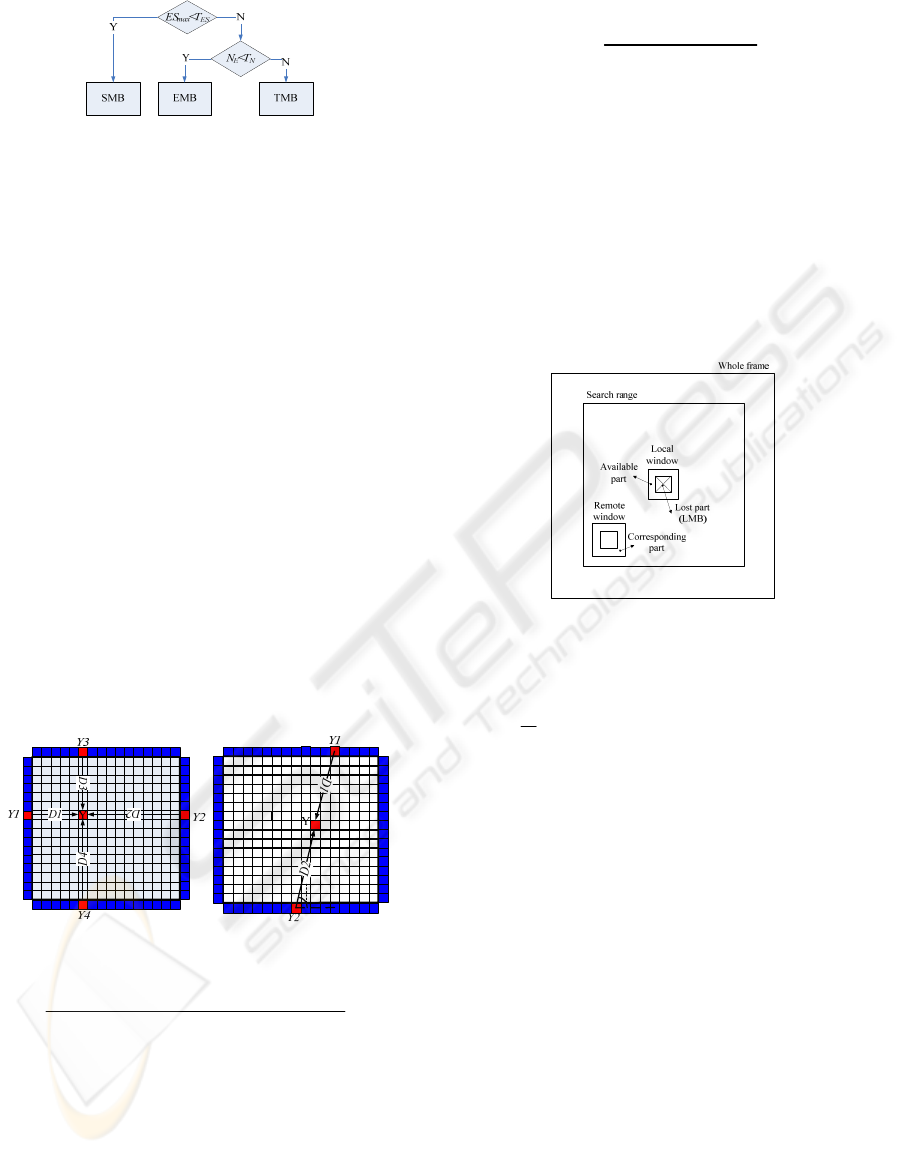
Figure 7: MB type decision in (Z Rongfu, 2004).

In Fig. 7, the ES

max

shown in Eq. 10 is the max-

imal value among all 8 edge strengths, and N

is the

count of strong directions, whose ES values are more

than 0.55*ES

max

. The threshold T

and T

are found

by trial and error, which are 3000 and 3 respectively,

2 fixed values for all cases. Since no statistics model

based measurement is considered, it is very hard to

achieve best image recovery in all cases.

0 7

max

(, ) (, ) (, )

max( ( , ),..., ( , ),..., ( , ))

ij N ij N ij N

ES ES i j ES i j ES i j

∈∈∈

∑∑∑

(10)

2.5 EC for Different MB Types

This section will briefly describe 3 different methods

for 3 different MBs respectively.

2.5.1 BI for SMB

Since pixels in SMB are basically constant or near so,

each pixel in LMB can be concealed by bilinear in-

terpolation using the nearest pixels from its 4 neigh-

bourhood boundaries. As the Fig. 8 shows, the in-

terpolated value of pixel Y is interpolated by Eq.11:

Figure 8: BI. Figure 9: DI

12 2134 43

1234

YDYDYDYD

DD D D

∗+∗+∗+∗

+++

(11)

2.5.2 DI for EMB

In order to preserve edge consistency, the LMB clas-

sified as EMB is interpolated along the edge direc-

tion described in section 2.2. Therefore, if the edge

of a certain direction k (corresponding to θ) is esti-

mated via Eq. 8 as a strong edge, then a series of

one-dimensional linear interpolation are carried out

along direction k to recover pixel values within the

LMB. This can be shown in Fig. 9 and Eq. 12.

1221

YD Y D

∗

+∗

(12)

2.5.3 BNM for TMB

Under the characteristics that TMB has some spatial

similarity compared with its NMB, a searching for

best neighbourhood matching (BNM) is performed

in this method. The best matching neighbour is the

one that minimizes the matching cost (MC), which is

a difference between the pixels of available part (1

layer of boundary pixels) in local window and the

pixels of corresponding part in remote window,

shown in Fig. 10.

Figure 10: BNM.

The mean square error (MSE) is used for mea-

surement of difference, which is shown in Eq.13.

(, ) _

(, ) [ (, ) ( , )]

i j available part

Cwijpijpisjt

∈

=∗−++

∑

(13)

where,

1, ( , ) ( , )

(, )

if both p i j and p i s j t are available

wi j

otherwise

⎧

⎨

⎩

(14)

and N is the number of calculated available pixels.

The region of s and t are both (-16x2, 16x2), which

denote that the search range is (16x5x16x5) square

area. After the best neighbourhood was found, the

lost part in local window is concealed by copy from

remote window.

3 EXPERIMENTS

The proposed error concealment algorithm is im-

plemented based on the H.264/AVC reference soft-

ware JM9.1. In order to evaluate our proposal, other

5 methods, BI in (Y.K.Wang, 2002), DI in (Jae-Won

Suh, 1997), BNM in (Zhou Wang, 1998), BI+DI in

(Dimitris, 2006) and BI+DI+BNM in (Z Rongfu,

2004) are also implemented. All 6 methods are tested

by 6 CIF sequences “foreman”, “bus”, “flower, “wa-

terfall”, “tempete”, and “stefan”. All tests are using

SIGMAP 2008 - International Conference on Signal Processing and Multimedia Applications

the same simulation setup. For each sequence, all

frames are encoded with intra encoding under H.264

baseline profile, and QP=28. For the MB loss, we

use FMO (flexible macroblock ordering) tool with 2

slices per frame in encoding (Stephan Wenger, 2003),

while 1 slice is lost for channel simulation. In Fig.

14(b), green MBs compose a lost slice while all 4

NMBs are available for each LMB. To evaluate im-

age recovery, both subjective and objective image

qualities are observed.

Fig. 11 shows the comparison of objective image

quality measurement, luminance PSNR for con-

cealed frames using different methods. A larger

PSNR value leads to a better image recovery. By

observing Fig. 13, some conclusions can be ob-

tained:

For different sequence, within DI, BI, and

BNM, different method wins the best recov-

ery, e.g., DI wins for foreman, BI wins for

bus, while BNM wins for flower. In other

words, in order to find a best image recovery,

an adaptive scheme is necessary.

II.

For adaptive method in (Dimitris, 2006),

compared with BI and DI, it dos not always

win the best recovery, such as bus, although

the difference with the winner is very small.

Same case was found in (Z Rongfu, 2004).

Compared with BI, DI, and BNM, method in

(Z Rongfu, 2004) does not always win the

best, such as foreman. However, for proposed

one, it always wins the best recovery.

Figure 11: Objective image recovery comparison.

Fig. 12 shows the subjective image quality com-

parison for flower sequence. Proposed method

achieves the best image recovery. It is easy to see

that, the optimal MB type for the flowers area should

be texture. However in algorithm of (Z Rongfu, 2004)

whose result is shown in Fig. 12(g), some LMBs in

flower area are regarded as SMB and recovered by

BI, which is a false MB type decision. In contrast,

our proposal avoided such false decision wel.

4 CONCLUSIONS

Considering there are 3 types of MBs in natural vid-

eo frame, i.e., TMB, EMB, and SMB, this paper

proposed an adaptive spatial error concealment,

which can choose 3 different methods for these 3

different MBs. For criterion of choosing, both edge

statistics measurement and intra prediction mode for

H.264 are taken into consideration. In terms of sub-

jective and objective image quality evaluation, expe-

riments show that the proposed method achieves the

best image recovery compared with previous work.

ACKNOWLEDGEMENTS

This work was supported by CREST, JST and Glob-

al-COE program of Japan.

REFERENCES

Jao-Won Suh, et al., 2002: Error concealment techniques

for digital TV. IEEE Trans. Broadcasting, Vol. 48

Yao.Wang, et al., 1998: Error control and concealment for

video communication: a review. Proceedings of IEEE,

pp947~997

Y.K.Wang, et al, 2002: The error concealment feature in

the H.26L test model. Proc. ICIP, vol.2, pp729~732

Jae-Won Suh, et al., 1997: Error concealment based on

directional interpolation. IEEE Trans. on consumer

electronics

Yan Zhao, et al, 2005: Spatial error concealment based on

directional decision and intra prediction. ISCAS

Dimitris, et al.: Enhanced error concealment with mode

selection. IEEE Trans. on circuits & sys for video tech

(2006)

Zhou Wang, et al., 1998: Best Neighborhood Matching:

An information loss based image coding systems.

IEEE Trans. on image processing

Z Rongfu, et al. 2004: Content-adaptive spatial error con-

cealment for video communication. IEEE Trans. on

consumer electronics, vol. 50, No.1

Thomas Wiegand, et al., 2003: Overview of the

H.264/AVC video coding standard. IEEE Trans. on

circuits and system for video technology

Stephan Wenger, 2003: H.264/AVC over IP. IEEE Trans.

on circuits and system for video technology

APPENDIX

In order to show the fact that 16x16 mode is more

suited for coding very smooth area, i.e., SMB, while

4x4 is well suited for area with significant detail, i.e.,

TMB, we did experiments to observe this.

AN ADAPTIVE SPATIAL ERROR CONCEALMENT FOR H.264/AVC VIDEO STREAM

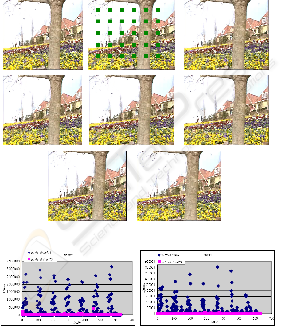
In our experiments, 2 CIF sequences, flower and

foreman, are observed. Fig 13 shows the result of

flower and foreman.

As the observation in Fig. 13 shows, MBs which

have lower ES

max

, usually are the MBs whose n

16x16

is more than n

4x4

. In the other hand, SMB always has

lower ES

max

, while TMB has higher of that. There-

fore, the observation successfully can match the fact

that generally 16x16 mode is suited for SMB while

4x4 mode is suited for TMB.

a) Original frame b) Damaged Frame, PSNR=13.37 c) BI only, PSNR=28.94

d) DI only, PSNR=28.29 e) BNM only, PSNR=29.66 f) Ref(Dimitris, 2006), PSNR=28.82

g) Ref(Z Rongfu, 2004),

PSNR=29.51

h) BI+DI+BNM in Proposed,

PSNR=30.6

Figure 12: Subjective image recovery comparison.

Figure 13: Intra mode observation.

SIGMAP 2008 - International Conference on Signal Processing and Multimedia Applications