CMB ANISOTROPIES INTERPOLATION

Svitlana Zinger

, Jacques Delabrouille

, Michel Roux

and Henri Maˆıtre

Eindhoven University of Technology, P.O. Box 513, 5600 MB Eindhoven, Netherlands

CNRS, Laboratoire APC, 10 rue Alice Domon et L´eonie Duquet, 75205 Paris Cedex 13, France

Ecole Nationale Sup´erieure des T´el´ecommunications, 46 rue Barrault, 75634 Paris Cedex 13, France

Keywords:

Interpolation, Cosmic Microwave Background, Binning, Kriging.

Abstract:

We consider the problem of the interpolation of irregularly spaced spatial data, applied to observation of

Cosmic Microwave Background (CMB) anisotropies.The well-known interpolation methods and kriging are

compared to the binning method which serves as a reference approach. We analyse kriging versus binning

results for different resolutions and noise level in the original data. Most of the time, kriging outperforms the

other methods for producing a regularly gridded, minimum variance CMB map.

1 INTRODUCTION

In this article we consider the problem of the inter-

polation of a set of data points for mapping Cosmic

Microwave Background (CMB) anisotropies.

CMB is a relic radiation emitted when the Uni-

verse was about 380,000 years old. Almost homo-

geneous and isotropic, it has small brightness irreg-

ularities of the order of one part per 100000, which

are imprinted by the tiny inhomogeneities which will

give rise to the large scale structures observable in the

Universe today, about 12 billion years later (Barreiro,

2000).

The observation of these anisotropies permits to

constrain the possible scenarios for describing the

content and evolution of our Universe. Many exper-

iments dedicated to these measurements have been

conducted in the past 20 years, included two space

missions and many ballon-borne or ground-based ex-

periments. ESA is planning launch the Planck space-

craft, for yet another space mission for observing

these signals with unprecedented accuracy. The scan-

ning strategy, which deﬁnes the scanning pattern on

the sky, is set by external constraints, which results in

general in somewhat irregularly gridded observations.

For this paper, we will investigate the problem of

interpolation on synthetic data sets which features a

few of the main difﬁculties encountered in real CMB

experiments.

2 DATA DESCRIPTION

The “data” used in this work is a simulated data set

covering a portion of the sky small enough to be

approximated by a tangent plane. The astrophysi-

cal signal comprises a 2-dimensional random ﬁeld

∆T

(~n) ≡

T(~n)−T

, where ~n is a unit vector on the

sphere. In addition, the map comprises emission from

about a thousand point sources, one of which is strong

enough to be representative of a bright planet. The

original sky map is convolved with a gaussian ker-

nel, to simulate the effect of the ﬁnite resolution of

the experiment. The original sky map is “observed”

in a number of points, arranged on fractions of circu-

lar scans. This is representative of the scanning of a

typical CMB instrument as Archeops. The real mea-

surements of CMB experiments are affected by noise.

This is modelled by adding a Gaussian noise with the

standard deviation in the range 0.2 to 1, so that the

SNR of measurements is typically between unity and

a few (units are arbitrary in the simulation). Although

the real cosmological measurements are made on a

sphere and therefore are determined using angles, we

consider local Cartesian coordinates. The simulated

measurements are the x,y coordinates and the corre-

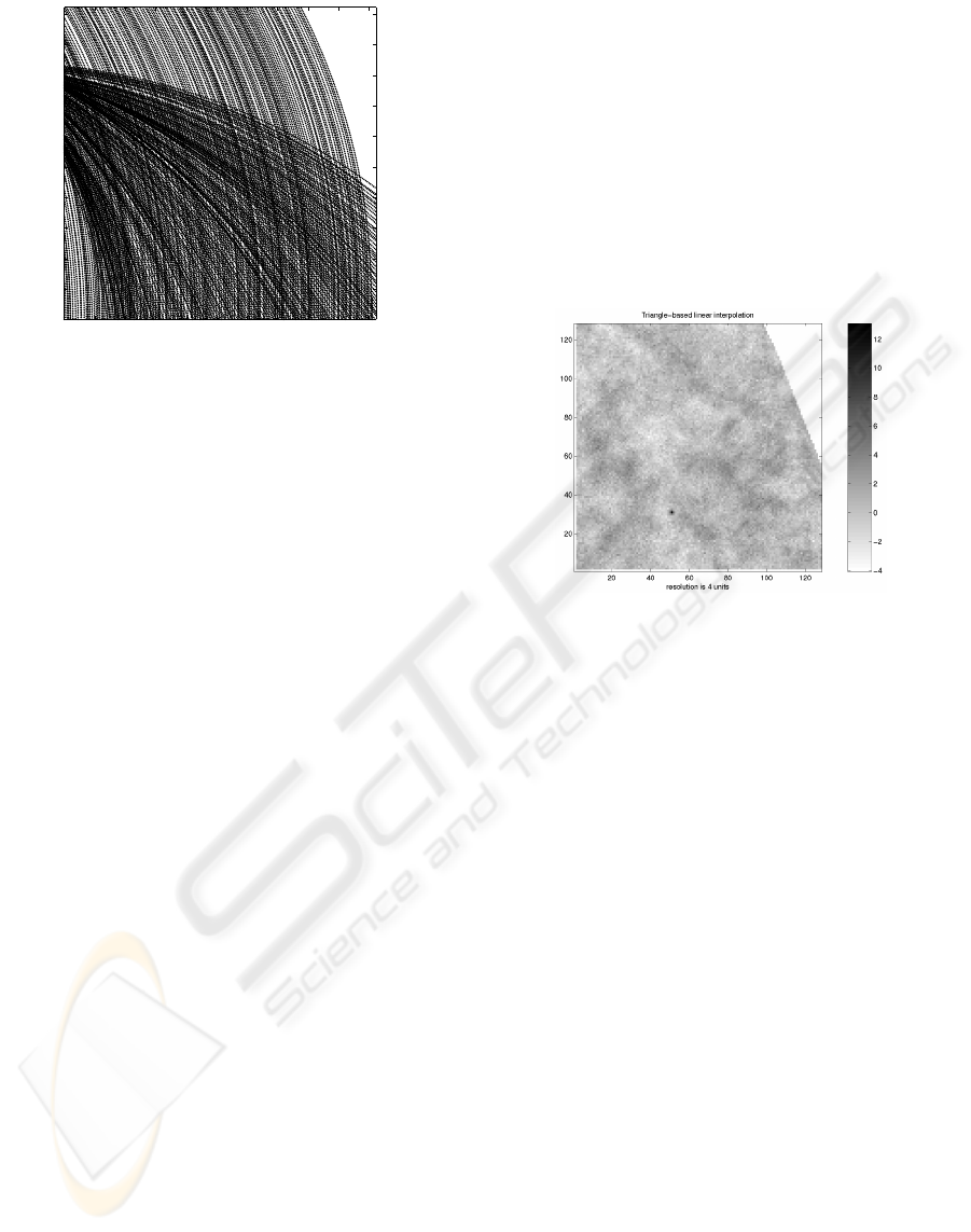
sponding anisotropy. Figure 1 shows x coordinates

plotted versus y coordinates of the data. From this

plot one can see the lines formed by the scanning pat-

tern. The total amount of points is 47914, 13 of them

correspond to the large point source in the data.

155

Zinger S., Delabrouille J., Roux M. and Maître H. (2009).

CMB ANISOTROPIES INTERPOLATION.

In Proceedings of the First International Conference on Computer Imaging Theory and Applications, pages 155-158

DOI: 10.5220/0001434401550158

 SciTePress

50 100 150 200 250 300 350 400 450 500

100

150

200

250

300

350

400

450

500

Figure 1: Simulated CMB measurements: x coordinates

versus y coordinates.

3 INTERPOLATION METHODS

We now present the interpolation experiments using

the simulated CMB data described above, with the

objective to identify the method best suited for resam-

pling the CMB data on a regular grid.

We speciﬁcally address the following problem.

For x and y coordinates varying between 0 and 511,

make an image with the size 128 × 128, 256 × 256

and 512× 512. This task considers the complete zone,

with low density of measures in some regions. This

task should also be performed on the data with noise.

We investigate several techniques that may be

used for the CMB measurements interpolation. We

consider triangle-based linear interpolation, kriging

and binning. Among those, we would like to choose

the best interpolation method according the root mean

square error (RMSE).

Binning, which simply consists in averaging mea-

surements “falling” in bins, is very simple and fast. It

is traditionally used for CMB observations.

Triangle-based interpolation is a method which

estimates the value of the observation at each sam-

pling point using the Delaunay triangulation, as a lin-

ear combination of data values at the vertices of the

appropriate triangle.

Kriging is similar to spline interpolation (Billings

et al., 2002) that can be presented as an energy min-

imization problem (Wolberg and Alfy, 2002). The

disadvantage of the cost function minimization is

the use of the coefﬁcient for the regularization term.

The change of this coefﬁcient will change the results

(Zinger et al., 2002).

The advantage of kriging over energy minimiza-

tion is that the parameters for kriging are obtained by

the analysis of the experimental variogram, that is ob-

tained from the original data, while the coefﬁcient for

the regularization term in the energy expression is the

parameter to tune.

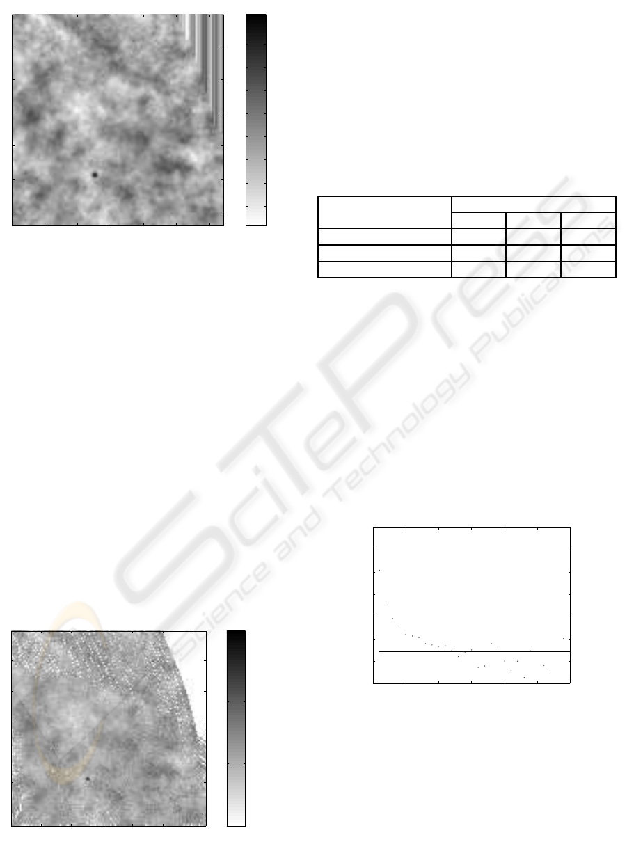
3.1 Linear Interpolation

Linear interpolation is based on Delaunay triangula-

tion of the original data. Triangle-based linear inter-

polation applies barycentric coordinates to the data at

the vertices of the triangle (Watson, 1992). Triangle-

based linear interpolation does not give good results

on the noisy data (Figure 2).

Figure 2: Triangle-based interpolation, x and y vary be-

tween 0 and 511, pixel size is 4 units.

3.2 Kriging

Kriging considers measurements as samples from a

realization of a stationary random process and analy-

ses the spatial behaviour of the corresponding param-

eters. The interpolation in this case consists of mak-

ing a weighted sum of the data points. The weights

are calulated using the variogram - a function that ex-

presses the spatial dependency between data. Most of

the research on the nature of the CMB anisotropies

characterizes them as a stationary random process of

the second order. Therefore the assumptions for krig-

ing (Cressie, 1991) are well veriﬁed for the CMB

data. Before using kriging it is necessary to determine

the three parameters of the variogram: the nugget, the

sill and the range (Billings et al., 2002). So the experi-

mental variogram is calculated, then these parametera

are obtained, and the used in the formula of the theo-

retical variogram.

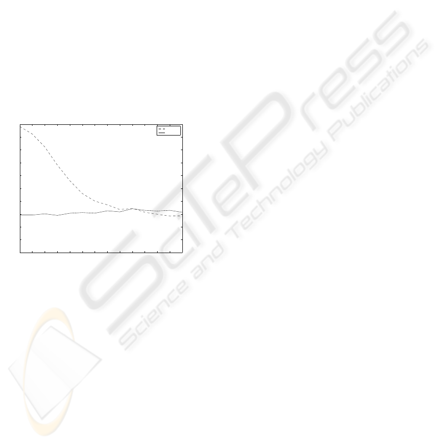
We perform the kriging interpolation on neighbor-

hoods of size 10 by 10 units. Kriging on a ﬁxed neigh-

borhood allows quick performance on large data sets

- it is an advantage for a real data interpolation.

The parameters estimated for the theoretical vari-

ogram from the noisy data are: range is 43, nugget is

1, sill is 1.8. An example of a resulting image is in

Figure 3.

IMAGAPP 2009 - International Conference on Imaging Theory and Applications

156

resolution is 4 units

Kriging: range is 43, nugget is 1, sill is 1.8

20 40 60 80 100 120

100

120

−2

−1

Figure 3: Kriging, x and y vary between 0 and 511, pixel

size is 4 units.

From the kriging results it is evident that the algo-

rithm suppresses noise.

3.3 Binning

A common and simple approach, that is often used in

astronomy, is binning. The method consists of aver-

aging the data values inside each bin centered around

a pixel to be computed. After having found the data

points located inside the area of a bin, the average of

these points values is attributed to the pixel. If there

are no data points inside a bin, then this pixel stays

empty, no value is assigned to it. If the bin size is

taken to be 2 units, then much less points fall inside

pixels. And when the bin size is 1 unit, then more than

80% of the pixels are empty and the pixels that have

data points, assigned to them, have just one point. So

in this case averaging is not possible. Figure 4 shows

results of binning.

resolution is 4 units

Binning on the noisy simulated CMB data

20 40 60 80 100 120

100

120

empty pixel

Figure 4: Binning, the resolution is 4 units.

4 COMPARISONS WITH THE

REFERENCE

Since our data is simulated, we can have a refer-

ence image to estimate the quality of the interpola-

tion methods. The root mean square errors (RMSE)

between the reference and interpolation results are in

Table 1.

Table 1: RMSE between the reference and the interpolation

results, x and y coordinates vary between 0 and 512.

Interpolation method Resolution

1 unit 2 units 4 units

Binning 0.9836 0.9238 0.6827

Linear 0.7152 0.7146 0.7085

Kriging 0.2930 0.2928 0.2900

From the RMSE values it is clear that kriging

gives better results than the other two interpolation

methods. The performance of binning becomes better

if the size of the pixel increases, since the larger the

bin, the more data points inside it. It is even possible

that binning gives better results than other methods

when the bin size is larger (and therefore, the resolu-

tion lower). Kriging has an advantage over binning,

because of using weighted average of the data and be-

cause the weights depend on the data statistics.

The quality of binning obviously depends on the

density of data points per regular grid pixel. Figure 5

demonstrates it.

0 5 10 15 20 25 30

0.2

0.4

0.6

0.8

1.2

1.4

Amount of points that fall inside a pixel

RMSE between the reference and binning result

Experiments on the data with noise, pixel size is 4x4

KRIGING

Figure 5: Hit counts versus RMSE for binning interpola-

tion. The horizontal line represents the RMSE value for

kriging with the same pixel size on the same data.

We can see that averaging on 10 or more pixels

often leads to the smaller errors than the ones of krig-

ing. So binning can outperform kriging only when the

density of points is quite high.

CMB ANISOTROPIES INTERPOLATION

157

5 KRIGING VERSUS BINNING:

PERFORMANCE ANALYSIS

From the previous results it is obvious that kriging

outperforms several other methods that we tried. The

reference method - binning - works worse especially

in the cases of small grid sizes, i.e. high resolution.

From the experiments presented above we can see

that kriging is the best, but binning can improve its

performance if the size of the pixel is enlarged, pos-

sibly at the price of reduced map resolution. When

the standard deviation of noise is 1, it is the case for

the Archeops acquisition system. We vary the pixel

size in order to see how it inﬂuences the interpolation

results.

Figure 6 demonstrate the RMSE measured be-

tween the reference and kriging or binning interpola-

tion results for different sizes of the pixel. Solid line

represent kriging, dashed - binning.

1 2 3 4 5 6 7 8 9 10 11 12 13 14

0.1

0.2

0.3

0.4

0.5

0.6

0.7

0.8

0.9

RMSE between the reference and the interpolation result

grid size

standard deviation for the noise is 1

binning

kriging

Figure 6: Kriging versus binning performance, standard de-

viation of noise is 1.

It is easy to see that the larger is the size of pixel,

the better is the binning result. The important advan-

tage of kriging is that its performance does not depend

on the choice of the resolution for the image. The

stronger is the noise, the larger pixel size is needed

in order to get binning results as good as the ones of

kriging. The grid size is 10 units when both methods

start having the same performance in the presence of

strong noise.

From the practical point of view, the size of the

grid equal to 7 or to 10 units is much too coarse. If

one wants to have the size of the grid the same as the

average density of the original scattered CMB data,

then it should be approximately 3 units.

6 CONCLUSIONS

Several methods can be used for the interpolation of

CMB anisotropies observations. These measurements

are irregularly distributed 3D points. In practice, they

are affected by noise and by other radiation sources.

We have considered the simulated data, composed by

the CMB anisotropiesand point sources and the noise.

For the data with noise we tried linear interpola-

tion, kriging and binning. Adding the noise compli-

cates the problem, especially because the range of the

noise is almost as large as the range of the data. In

this case an interpolation technique should be able

to decrease the effect of noise as much as possible.

The best results are obtained with the kriging tech-

nique, because it allows to take the noise into account

through the parameters of the variogram.

Binning is often used in astronomy, it averages the

values of the data inside each pixel and so can de-

crease the noise. The disadvantage is that the density

of data points should be at least ten times higher than

the density of the regular grid in order to get good re-

sults. It is also desirable for binning to have evenly

distributed data points. Taking binning as the ref-

erence method, we make a detailed comparison be-

tween this method and kriging. We ﬁnd that these

two methods can be equally good when the regular

grid size of the image to ﬁnd is very coarse. Oth-

erwise, for acceptable grid sizes kriging outperforms

binning.

REFERENCES

Barreiro, R. B. (2000). The cosmic microwave background:

state of the art. New Astronomy Reviews, 44:179–204.

Billings, S. D., Beatson, R. K., and Newsam, G. N. (2002).

Interpolation of geophysical data using continuous

global surfaces. Geophysics, 67(6):1810–1822.

Cressie, N. A. (1991). Statistics for spatial data. A Wiley-

Interscience publication.

Watson, D. F. (1992). Contouring: a guide to the analysis

and display of spatial data. Pergamon Press.

Wolberg, G. and Alfy, I. (2002). An energy minimization

framework for monotonic cubic spline interpolation.

Journal of Computational and Applied Mathematics,

143(2):145–188.

Zinger, S., Nikolova, M., Roux, M., and Maˆıtre, H. (2002).

3d resampling for airborne laser data of urban areas.

In Proc. ISPRS Symposium PCV’02, volume XXXIV,

pages 418–423.

IMAGAPP 2009 - International Conference on Imaging Theory and Applications

158