VARIABLE SUBSET SELECTION FOR BRAIN-COMPUTER

INTERFACE

PCA-based Dimensionality Reduction and Feature Selection

N. S. Dias

, M. Kamrunnahar

, P. M. Mendes

, S. J. Schiff

and J. H. Correia

Dept. of Industrial Electronics, University of Minho, Campus Azurem, 4800-058 Guimaraes, Portugal

Dept. of Engineering Sciences and Mechanics, The Pennsylvania State University, University Park, PA 16802, U.S.A.

Keywords: BCI, EEG, Feature selection.

Abstract: A new formulation of principal component analysis (PCA) that considers group structure in the data is

proposed as a Variable Subset Selection (VSS) method. Optimization of electrode channels is a key problem

in brain-computer interfaces (BCI). BCI experiments generate large feature spaces compared to the sample

size due to time limitations in EEG sessions. It is essential to understand the importance of the features in

terms of physical electrode channels in order to design a high performance yet realistic BCI. The VSS

produces a ranked list of original variables (electrode channels or features), according to their ability to

discriminate between tasks. A linear discrimination analysis (LDA) classifier is applied to the selected

variable subset. Evaluation of the VSS method using synthetic datasets selected more than 83% of relevant

variables. Classification of imagery tasks using real BCI datasets resulted in less than 16% classification

error.

1 INTRODUCTION

Brain-Computer Interfaces (BCI) enable people to

control a device with their brain signals (Wolpaw et

al., 2000). BCIs are expected to be a very useful

tool for impaired people both in invasive and non-

invasive implementations. Non-invasive BCI

operation commonly uses electroencephalogram

(EEG) from human brain for the ease of

applicability in laboratory set ups as well as in

patient applications. Datasets are generally high-

dimensional, irrespective of the types of features

(frequency band power, event-related

desynchronization (ERD), movement-related

potentials (MRP), event-related potentials (e.g.

P300), etc.) extracted from EEG, if no previous

knowledge about those features is considered. The

low ratio of the number of samples to the number of

variables is described as the curse of dimensionality

(Duda et al., 2000). Frequently, in a BCI experiment,

it is not easy to increase the number of samples to

compensate for high-dimensionality. On the other

hand, a variable subset calculation is feasible when

few variables are relevant.

The variables in a dataset can be divided into

irrelevant, weakly relevant and strongly relevant

variables (John et al., 1994). A good subset should

include all the strongly relevant variables and some

of the weakly relevant ones. The variable subset to

choose should minimize the generalization error (i.e.

cross-validation error). Typically, the term ‘feature’

is used in the literature (Yu and Liu, 2004) instead of

‘variable’. Nevertheless, we here use the latter to

avoid confusion about the dimensions of the dataset

(electrode channels) and the characteristic features

(e.g. band power, MRP) extracted from EEG raw

signals.

This work proposes a feature selection method

based on a different formulation of Principal

Component Analysis (PCA), introduced in (Dillon,

1989) that accommodates the group structure of the

dataset. In the PCA framework, data dimensionality

reduction methods typically use the selected

principal components (PC) as a lower-dimensional

representation of original variables, for

discrimination purposes (Dillon et al., 1989;

Kamrunnahar et al., 2008). However, the proposed

work suggests that the dimensionality reduction

should take place on the original variable space

instead of the components, since it becomes more

obvious which original variables are really relevant.

The datasets from each subset of variables undergo

Dias N., Kamrunnahar M., Mendes P., Schiff S. and Correia J. (2009).

VARIABLE SUBSET SELECTION FOR BRAIN-COMPUTER INTERFACE - PCA-based Dimensionality Reduction and Feature Selection.

In Proceedings of the International Conference on Bio-inspired Systems and Signal Processing, pages 35-40

DOI: 10.5220/0001533200350040

 SciTePress

linear discriminant analysis (LDA) for classification.

The best subset in discriminating between task

performances, for each subject, is evaluated by a

cross-validation error.

We evaluated the proposed VSS method through

both synthetic and real datasets. A synthetic dataset

enabled us to evaluate this method in a controlled

environment and simulated the 3 levels of variable

relevance mentioned above. The real datasets were

generated from movement-related potentials (MRP)

as EEG responses to movement imagery tasks

(Babiloni et al., 1999). Four subjects were submitted

to these experiments and no subject had previous

BCI experience. The lowest cross-validation error

for each subject and the corresponding number of

variables selected were assessed.

2 EXPERIMENTAL DESIGN

2.1 Symthetic Data

Among all variables p in the synthetic dataset, q

relevant and p-q irrelevant Gaussian distributed

variables were generated. All the generated variables

had the same standard deviation σ. In order to best

simulate a typical multivariate dataset, the relevant

features were generated in pairs with correlation

between variables. In this way, the variables are

more discriminative if considered together. The first

variable in each pair is considered as the

predominant variable since its mean has distance d

between groups. The distribution parameters were

set similarly to (Lai et al., 2006). Pairs of correlated

variables were generated until the quantity of

relevant variables is reached. The remaining p-q

variables (i.e. discrimination irrelevant) were

generated from the same Gaussian distribution (no

mean difference) for both groups. Four different

datasets were generated with 80 samples: p=79 and

q=6; p=79 and q=12; p=40 and q=6; p=40 and q=12.

The first 2 datasets were intended to simulate the

high dimensional/low sample size problem. The last

2 represent a lower high-dimensional space. The

standard deviation σ was set to 2.5 in all datasets.

The mean difference d was set to be equal to σ to

simulate group overlapping. The values of both

distribution parameters were set to best approximate

the real variables extracted from the EEG data

collected.

2.2 EEG Data

Four healthy human subjects, 25 to 32 years old,

three males and one female, were submitted to 1

session each of motor imagery. The experiments

were conducted under Institutional Review Board

(IRB) approval at Penn State University.

Each session had 4 runs of 40 trials each. Each

subject was instructed to perform one of 4 tasks in

each trial. The tasks were tongue, feet, left hand and

right hand movement imageries. The following 2

imagery task discrimination cases were considered

for VSS algorithm evaluation: tongue vs. feet; left

hand vs. right hand. After the first 2 s of each trial, a

cue warned the subject to be prepared and 1 s later, a

cue about the required mental task was presented to

the subject. The subject was instructed to perform

the task in the 4 s after the cue.

Data were acquired from 9 electrodes according to

the standard 10-20 system (F3, Fz, F4, C3, Cz, C4,

P3, Pz, P4). All electrodes were referenced to linked

earlobes. Data were digitized at 256 Hz and passed

through a 4th order 0.5-60 Hz band-pass filter. Each

channel’s raw EEG signal was epoched from the cue

time point (0 s) to 4 s after the cue. The epoch was

subdivided in 1 s time windows with no overlap (4

time windows). Each epoch was low-pass filtered at

4 Hz with an 8th order Chebyshev type I filter.

Then, the filtered 256 points time series was down

sampled to be 10 points long. The Matlab

“decimate” function was used to accomplish both

the filtering and down sampling. Only the 1

-8

data

points of the resultant time series form the feature

vector for each time window. The last 2 points of the

time series were discarded because they seemed to

be irrelevant on previous analyses. The feature

matrix of each time window had 72 variables (8

features from each of the 9 electrodes) and 80

samples.

3 VARIABLE SUBSET

SELECTION

The proposed VSS algorithm can be partitioned in 3

sequential procedures. Initially, the dataset

dimensionality is reduced through a formulation of

PCA that accommodates the group structure of the

dataset (Dillon, 1989). Once the number of variables

is reduced, the remaining variables are ranked

according to their discrimination ability. Finally a

cross-validation procedure is applied in order to

determine the optimum subset of variables to select.

BIOSIGNALS 2009 - International Conference on Bio-inspired Systems and Signal Processing

3.1 Dimensionality Reduction

The original feature matrix Y has samples in rows

(n) and variables (p) in columns (p < n-1). The PCs

are linear projections of the variables onto the

orthogonal directions that best describe the dataset

variance independent of any group structure that

might be present in the data. Initially, the p PCs in

n×p

are calculated through singular value

decomposition (SVD) of Y. Although the PCs are

already organized by decreasing order of total

variance accounted for, this order is optimized for

orthogonality rather than discrimination between

groups. In order to compensate for this and take the

data group structure into account, the components

should be ordered according to the across group

variance (AGV) score (Dias, 2007), instead of the

eigenvalues λ

order that account for the total

variance. The AGV score is used to rank each

component in terms of the between group variance

instead of the total variance. The AGV score is

calculated according to (1) and its implementation is

detailed in the appendix.

i Between i

AGV

(1)

Between

represents the between group covariance

matrix (see appendix for calculation details) and v

represents the i

eigenvector of Ψ.

The dimensionality reduction results from the

truncation of the component matrix (U), previously

ordered according to the AGV scores. The

truncation criterion was set to 80% (unless otherwise

noted) of the cumulative sum (in decreasing order of

the AGV scores) of every component’s AGV. The

truncated version of U (U

n×k

), with k < p

components, is a lower dimensional representation

of the original variable space in Y and is often used

as a reduced feature matrix (Kamrunnahar, 2008).

Although each component in U is a linear

combination of all the original variables in Y, it is

not always evident what each component means in

the original variable space (Jolliffe, 2002). Hence,

the original k variables (Y

n×k

) which have the most

variance accounted for in the truncated component

space (U

n×k

) are used as a representation of the

original variable space Y. The vector sub keeps the

indices of the k variables that were kept after this

dimensionality reduction (see appendix for details).

Therefore, at the end of this stage, the

dimensionality of the dataset has been reduced from

p to k.

3.2 Variable Ranking

On the one hand, 2 different variables might have

the same variance accounted for the k PCs but have

different importance as discriminators (predictor in

LDA). We indeed found in the current analyses, for

both synthetic and real BCI datasets, that variables

with high variance accounted for the k PCs were

poor discriminators. On the other hand, a variable

that is a good discriminator is expected to have high

variance in the k PCs that were kept in the previous

subsection. Therefore, in this 2

procedure, a ranked

list of the variables in sub is calculated according to

their discrimination ability. The rank, in (2),

computes the multivariate distance penalization

observed when each variable at a time is removed

from the subset of k variables.

()

rank Y D D

−

, jsub∈

(2)

The multivariate distance D is calculated as in (3).

and Μ

are the multivariate means of groups 1

and 2 respectively, and Ψ

is the covariance matrix

of the k selected variables. D

-j

is calculated by

excluding the variable j to calculate the multivariate

distance.

12 12

()()

⎡

⎤

=Μ−Μ ΨΜ−Μ

⎣

⎦

(3)

The output of this procedure is the reorganized

version of sub with variables in descending order

according to rank(Y

In order to show the importance of the

dimensionality reduction step in eliminating non-

relevant variables, all the p variables in Y were

ranked and classified in a separate cross-validation

step where the 1

procedure (i.e. dimensionality

reduction) was omitted (figures 1 and 3).

3.3 Cross-Validation

Once the subset of variables sub is ordered

according to (2), an LDA classifier is applied

iteratively on each feature matrix Y

sub(f)

containing

the f top most ranked variables in sub, for f=1,…,k.

The leave-one-out error rate (LOOR) is calculated in

each iteration. The lowest LOOR value achieved

determines which subset of variables opt (opt ⊂ sub)

is optimal according to this approach (results in

figures 1 and 3).

A different approach of Fisher Discriminant

Analysis (Schiff, 2005) that was robust on

spatiotemporal EEG pattern discrimination was

applied. The canonical discrimination functions Z

are the result of a linear transformation of original

VARIABLE SUBSET SELECTION FOR BRAIN-COMPUTER INTERFACE - PCA-based Dimensionality Reduction and

Feature Selection

data Y according to (4). The discrimination

coefficients of each i

canonical discrimination

function are denoted by the columns of b

()

isubji

Yb=

(4)

The group membership prediction was based on

the posterior probability π

as the probability that

the data of a given value z came from group g

(Dias, 2007). The highest π

value (g ∈ {1,2}: only

left vs. right hand movements and tongue protrusion

vs. feet movement imagery discriminations were

assessed) was the predicted group membership for

posterior calculations.

The discrimination quality was assessed by

LOOR and Wilks’ statistic W. Further details on the

classification method can be found in (Dias, 2007).

4 RESULTS

The feature selection process on the synthetic data

was evaluated for 4 different cases of number of

features p and different number of relevant features

q. Two cases are illustrated in figure 1. The 1

case

(p=40; q=6) at figure 1 left plot achieved 7.5 % of

LOOR and Wilks’ statistic W=0.33 which is very

significant since the 99 % confidence value W99 (W

is chi-squared distributed with p×(n-1) degrees of

freedom) for this statistic is 0.74. All 6 relevant

variables were selected for the optimal subset

(minimum LOOR). The 2nd case (p=40; q=12)

achieved 0 % LOOR for 10 variables (10 relevant

features out of 12 were selected and all the

predominant ones were selected) and W=0.16

(W99=0.75). The 3rd case (p=79; q=6) at figure 1

right plot reached 3.7 % LOOR for 5 variables (all

the predominant variables were selected) and

W=0.23 (W99=0.83). Finally the 4th case (p=79;

q=12) reached 3.7% LOOR for 14 variables (all

relevant variables were selected plus 2 irrelevant

ones) and W=0.14 (W99=0.69).

The FSS algorithm was also tested in real data

from 4 subjects which achieved between 11.4 % and

29.1 % LOOR (each subject’s best time window) for

left vs. right imagery (figure 2 left plot). During

tongue vs. feet imagery performance, the LOOR was

between 15.2 % and 30.4 % (0-1 s time window), as

seen on figure 2. The best occurrence from each

discrimination case is depicted on figure 3. In both

cases 4 variables were selected as the optimal subset.

In JF’s left vs. right performance (figure 3 left plot)

analyses, features from C4, Pz, F3 and Fz channels

were selected. In JI’s tongue vs. feet performance

(figure 3 right plot) analyses, features from P3, C3,

Cz and Pz channels were selected. On figure 1 as

well as figure 3, the variables selected until the

minimum LOOR is reached (opt) are considered

relevant and all the following variables selected are

considered irrelevant.

2 4 6 8 1

0.05

0.1

0.15

0.2

0.25

#variables selected j

LOOR(%)

p=40 q=6

VSS steps 1+2

VSS step 2

opt

85%

5 10 15 20

0.1

0.2

0.3

0.4

#variables selected j

LOOR(%)

p=79 q=6

VSS steps 1+2 VSS step 2

opt

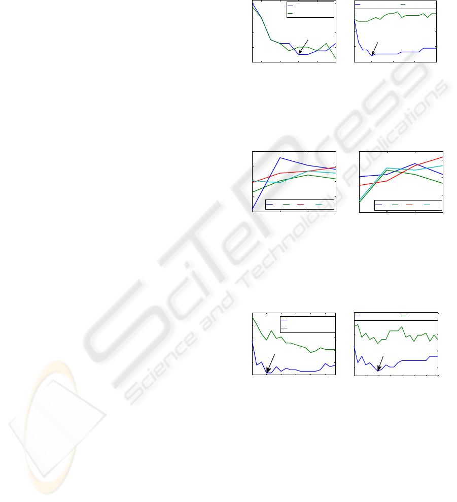
Figure 1: Plots of LOOR vs. number of variables selected

from sub for both the VSS algorithm (blue line) and VSS

2nd step separately (green line). Two different cases were

illustrated for q relevant variables out of p variables.

1 2 3 44

0.1

0.2

0.3

0.4

0.5

window last time point (s)

LOOR(%)

left vs. right performance

JF JI JM SS

1 2 3 4

0.1

0.2

0.3

0.4

window last time

oint

(

)

LOOR(%)

tongue vs. feet performance

JF JI JM SS

Figure 2: LOOR variation through 4 time windows (1-4 s

after cue) for all 4 subjects (JF, JI, JM and SS) for left vs.

right movement imagery performance (left plot) and

tongue vs. feet movement imagery performance (right

plot).

1 4 7 10 13 16 1

0,1

0,3

0,5

#variables selected j

LOOR(%)

JF left vs. right (window 0-1 s)

VSS steps 1+2

VSS step 2

opt

1 4 7 10 13 16 19 22

0.2

0.3

0.4

0.5

#variables selected j

LOOR(%)

JI tongue vs. feet (window 0-1 s)

VSS steps 1+2 VSS step 2

opt

Figure 3: LOOR vs. number of variables selected for JF

(left plot) and JI (right plot) in time window 1.

5 DISCUSSION

AND CONCLUSIONS

The goal of this VSS approach is to find few

relevant variables for discrimination in a high-

dimensional variable space. The results with

synthetic datasets reveal that this goal is feasible: at

least 83% of the relevant variables were selected for

the optimal subsets; 100% of the predominant

BIOSIGNALS 2009 - International Conference on Bio-inspired Systems and Signal Processing

variables were selected for all optimal subsets; all

the discriminations reached less than 7.5% LOOR

and were very significant. The 1

and 2

cases show

that this approach is also applicable for lower

dimensional variable spaces (p=40;N=80) as well as

high-dimensional ones (3

and 4

cases). As shown

in figure 1 for p=79 and figure 3 the LOOR is much

larger when only the 2

step of VSS is applied alone

(green line) to all original variables, than the LOOR

achieved when both steps are applied jointly (blue

line). Although the LOOR increase in the absence of

the 1

step is less evident for p=40 (figure 1), the

optimal solution is still achieved when both steps are

applied jointly. Therefore, it can be concluded from

these results that the proposed algorithm reduces the

number of variables efficiently as well as decreases

the discrimination error.

Real BCI data results, on figure 2, show three

good discrimination cases (LOOR lower than 16%)

for three different subjects. The presence of just few

relevant variables in these BCI datasets seems likely

once 4 (subject JF) and 7 (subject JI) variables out of

72 were selected for the optimal subset in figure 3.

As suggested in the literature (Babiloni, 1999), for

all cases but one in figure 2, the best time window

for classification appears to be the first second after

cue.

Our findings show a novel mean to down-select

variables in BCI that accomplishes both

discriminative power and dimensionality reduction.

Such a strategy is valuable in decreasing the

computational complexity of neural prosthetic

applications.

ACKNOWLEDGEMENTS

N. S. Dias is supported by the Portuguese

Foundation for Science and Technology under Grant

SFRH/BD/21529/2005 and Center Algoritmi. S. J.

Schiff and M. Kamrunnahar were supported by a

Keystone Innovation Zone Grant from the

Commonwealth of Pennsylvania, and S. J. Schiff by

NIH grant K02MH01493.

REFERENCES

Babiloni, C., Carducci, F., Cincotti, F., Rossini, P.M.,

Neuper, C., Pfurtscheller G., Babiloni, F., 1999.

Human movement-related potentials vs

desynchronization of EEG alpha rhythm: A high-

resolution EEG study. In NeuroImage, vol. 10, pp.

658-665.

Dias, N.S., Kamrunnahar, M., Mendes, P.M., Schiff, S.J.,

Correia, J.H. Customized Linear Discriminant

Analysis for Brain-Computer Interfaces. In Proc.

CNE '07 IEEE/EMBS 2-5 May 2007, pp. 430-433.

Dias, N.S., Kamrunnahar, M., Mendes, P.M., Schiff, S.J.,

Correia, J.H. Comparison of EEG Pattern

Classification Methods for Brain-Computer Interfaces.

In Proc.29th EMBC 22-26 Aug 2007, pp.2540-2543.

Dillon, W.R., Mulani, N., Frederick, D.G., 1989. On the

Use of Component Scores in the Presence of Group

Structure. JOURNAL OF CONSUMER RESEARCH,

vol. 16, pp. 106-112.

Duda, R.O., Hart, P.E., Stork, D.G., 2000. Pattern

Classification. Wiley.

John, G.H., Kohavi, R., Pfleger, K., 1994. Irrelevant

Features and the Subset Selection Problem. In Proc.

11th Int. Conf. Machine Learning, 121-129.

Jolliffe, I.T., 2002. Principal Component Analysis,

Springer 2

edition.

Kamrunnahar, M., Dias, N.S., Schiff, S.J. Model-based

Responses and Features in Brain Computer Interfaces.

In Proc. 30

IEEE EMBC 20-25 Aug 2008, pp.4482-

4485.

Lai, C., Reinders, M.J.T., Wessels, L., 2006. Random

subspace method for multivariate feature selection.

Pattern Recognition Letters, no.27, pp.1067-1076.

Schiff, S.J., Sauer, T., Kumar, R., Weinstein, S.L., 2005.

Neuronal spatiotemporal pattern discrimination: The

dynamical evolution of seizures. NEUROIMAGE, 28

ed, pp. 1043-1055.

Wolpaw, J.R., McFarland, D.J., Vaughan, T.M., 2000.

Brain–Computer Interface Research at the Wadsworth

Center. IEEE TRANSACTIONS ON REHAB.

ENGINEERING, vol. 8, no. 2, pp. 222-226.

Yu, L., Liu, H., 2004. Efficient feature Selection via

Analysis of Relevance and Redundancy. Journal of

Machine Learning, no. 5, pp. 1205-1224.

APPENDIX

This section details the dimensionality reduction

implemented on the proposed variable selection

algorithm. The algorithm presented on the bottom of

this section enumerates every command of this

procedure.

On the line 1 of the algorithm, Y is decomposed

through SVD into 3 matrices: U

n×p

(component

orthogonal matrix), S

p×p

(singular value diagonal

matrix) and V

p×p

(eigenvector orthogonal matrix).

The eigenvalues vector

is calculated on line 2 as

the diagonal of S

. The AGV score is calculated for

every PC through lines 4 to 6.

Once it is considered that both groups to

discriminate have the same covariance matrix, the

pooled covariance matrix should be calculated as the

within group covariance matrix Ψ

Within

VARIABLE SUBSET SELECTION FOR BRAIN-COMPUTER INTERFACE - PCA-based Dimensionality Reduction and

Feature Selection

112 212

(1) ( 1) 2

Within

nnnnΨ=−Ψ+−Ψ−−

and n

are respectively the covariance matrix and

number of samples belonging to the i

group.

Considering Ψ as the total covariance matrix, the

between groups covariance matrix Ψ

Between

calculated as:

etween Within

Ψ=Ψ−Ψ

On line 7, the vector rAGV is a version of AGV

in descending order. On lines 8 and 9,

and the

columns of V are similarly reordered in r

and rV

respectively, to match rAGV. Note that AGV is

originally ordered according to the descending order

of the eigenvalues

(line 5). The reordered AGV

indices are kept in dpc, which stands for

‘discriminative PCs’, where rAGV=AGV

dpc

Each component’s percentage of the sum of all

AGV scores is calculated on line 10. The number of

components k out of p to maintain determines the

truncation to be performed in U. k is calculated on

line 11 as the number of elements of %rAGV whose

cumulative sum is higher than the component

selection criterion (δ).

Considering the spectral decomposition

property of the covariance matrix:

iii

Ψ=

∑

The columns of V are the eigenvectors v

. The

diagonal values of Ψ give the variance of the

variables in Y accounted for the p PCs, as well as

TruncVar

gives the ‘truncated’ variance of variable j

accounted for the k PCs that were kept for

dimensionality reduction.

On lines 15 and 16, the vector rTruncVar is a

descending ordered version of TruncVar and the

indices of the k top most variables in rTruncVar are

copied into the subset of variables sub.

Input Data: Y, Ψ

BETWEEN

, δ

Output Data: sub

1. [U,S,V

] = SVD(Y);

2. λ = diag(S

);

3. p = # columns of Y;

4. for i=1 to p do

5. AGV

= V

×Ψ

BETWEEN

×V

/λ

6. end for

7. [rAGV,dpc] = sort AGV in

descending order

8. rλ = λ

dpc

{λ is reordered to

match rAGV}

9. rV = V

dpc

{V is reordered to

match rAGV}

10. %rAGV = 100*rAGV / Σ

i=1,..,p

rAGV

11. k = number of first %rAGV

elements whose cumulative sum > δ

12. for j=1 to p do

13. TruncVar

= Σ

i=1,..,k

rλ

×rV

14. end for

15. [rTruncVar,Index] = sort

TruncVar in descending order

16. sub = 1st k elements in Index

BIOSIGNALS 2009 - International Conference on Bio-inspired Systems and Signal Processing