AN EXPERIMENTAL COMPARISON OF NONHOLONOMIC
CONTROL METHODS
Kang-Zhi Liu
Department of Electrical and Electronics Engineering, Chiba University, Chiba, Japan
Keywords:
Parking benchmark, Khennouf-Wit method, Astolfi’s method, Sordalen-Egeland method, Ikeda-Nam-Mita
method, Jiang’s method, Liu-Sampei method.
Abstract:
Although numerous nonholonomic control methods have been proposed, few is known about the advantages
and disadvantages of each method. So in this paper an automatic parking system is used as a benchmark to
test several typical nonholonomic control approaches experimentally. The emphasis is put on the applicability
and control performance.
1 INTRODUCTION
Since the last decade nonholonomic control has been
studied extensively and numerous methods have been
proposed. However, no experimental comparison was
reported up to date to the knowledge of the author. So
in this paper the automatic parking problem will be
used as a benchmark to test several typical nonholo-
nomic control approaches experimentally.
The methods to be tested are (1) Khennouf-
Wit method (H.Khennouf and Wit, 1996), (2)
Astolfi’s method (Astolfi, 2000), (3) Sordalen-
Egeland method (Sordalen and Egeland, 1995), (4)
Ikeda-Nam-Mita method (Ikeda et al., 2000), (5)
Jiang’s Method (Jiang, 2000) and (6) Liu-Sampei
method (Sampei and et al., 1995; Liu et al., 2006).
The following specifications are used for compar-
ison: (1) applicability to automatic parking subject
to steering angle and parking space constraints, (2)
safety, (3) convergence performance of each variable,
(4) oscillatory behaviour during the parking control
process.
2 MODEL AND EXPERIMENT
SET-UP
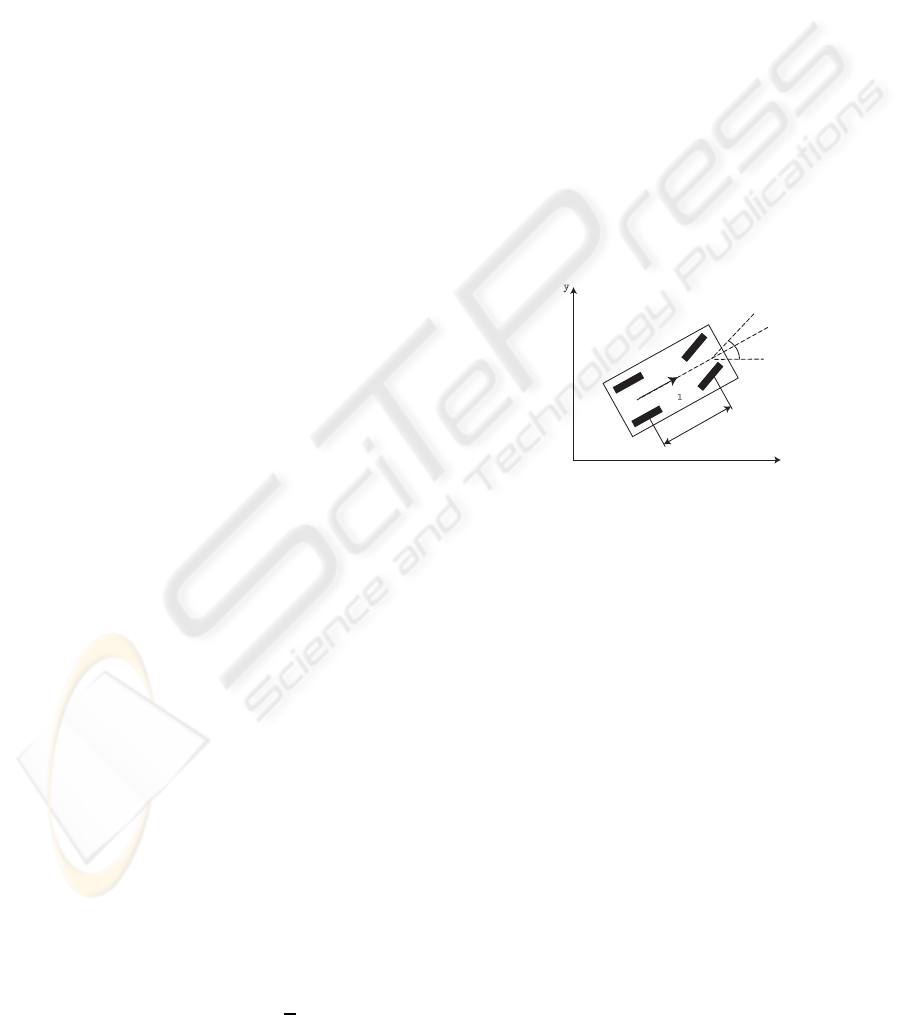
The plant is a rear-drive 4-wheeled car illustrated in
Fig. 1. Subject to the assumption that no side slip
occurs, the kinematic model is described by
˙x = u
1
cosθ, ˙y = u
1
sinθ,
˙
θ = u
1
1
L
tanφ (1)
x,y
u
1
L
x
y
0
θ
φ
Figure 1: Model of 4-wheeled car.
in which L denotes the wheel base, (x,y) is the posi-
tion of the center of rear wheel, θ is the orientation
angle with respect to x axis. Further, φ and u
1
denote
the steering angle and driving velocity respectively.
Here
η = tanφ
and the driving velocity u
1
are regarded as the control
input.
As real cars are subject to limitation of steering
angle, the steering angle will saturate when the de-
signed steering angle surpasses this limitation. That
is, when the limit of steering angle is given by
φ ∈ [−φ
max
,φ
max
], φ
max
> 0 (2)
the real input η becomes
η =
η
∗
, |φ| ≤ φ
max
sgn(η
∗
)|η
max
|, |φ| > φ
max
(3)
where η
∗
= tanφ
∗
denotes the designed input and
η
max
= tanφ
max
.
208
Liu K. (2009).
AN EXPERIMENTAL COMPARISON OF NONHOLONOMIC CONTROL METHODS.
In Proceedings of the 6th International Conference on Informatics in Control, Automation and Robotics - Robotics and Automation, pages 208-213
DOI: 10.5220/0002205802080213
Copyright
c
SciTePress
Applying the following variable transformation
z
0
= x, z
1
= y, z
2
= tanθ (4)
as well as input transformation
v
0
= u
1
cosθ
v
1
=
1
L
η
∗
(1+ tan
2
θ)u
1
(η
∗
= tanφ)
(5)
to the system (1) leads to a 3rd order chained system:
˙z
0
= v
0
, ˙z
1
= z
2
v
0
, ˙z
2
= v
1
. (6)
Most of the 6 methods are built with respect to this
chained system.
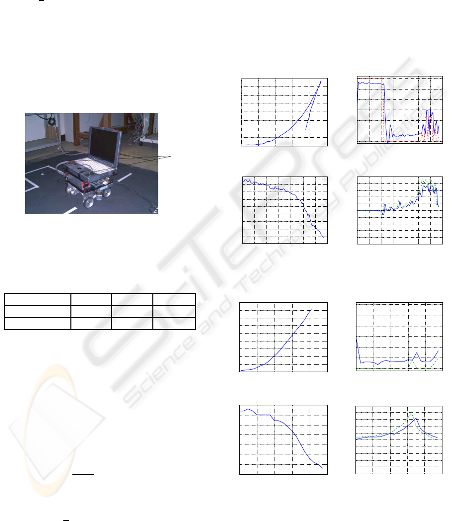
The prototype motor car used in experiment is
shown in Fig.2, in which the garage and road are in-
dicated by the white lines.
LED
Figure 2: Experiment system.
Numerous parking experiment have been con-
ducted and two sets of them will be shown (Table 1).
Table 1: Initial values.
x(0) y(0) θ(0)
Experiment 1 37[cm] 20[cm] 85[deg]
Experiment 2 41[cm] 16[cm] 33[deg]
In experiments, the designed driving velocity and
steering angle are applied to their closed loop systems
as reference input. Also in all figures of responses
the solid, dotted lines show the measured data and the
computed reference, respectively.
3 KHENNOUF-WIT METHOD
The input is given by
v =
v
0
v
1
= 2f
S(z)
W(z)
−z
2
z
0
− k
z
0
z
2
(7)
in which S(z) and W(z) are
S(z) = z
1
(t) −
1
2
z
0
(t)z
2
(t), W(z) = z
2
0
+ z
2
2
. (8)
The closed loop system satisfies
W = W(z(0))exp(−2kt), S = S(z(0))exp(− ft) (9)
when this input is applied to system (6). Therefore,
W,S, z
0
,z
1
,z
2
converge to zeros.
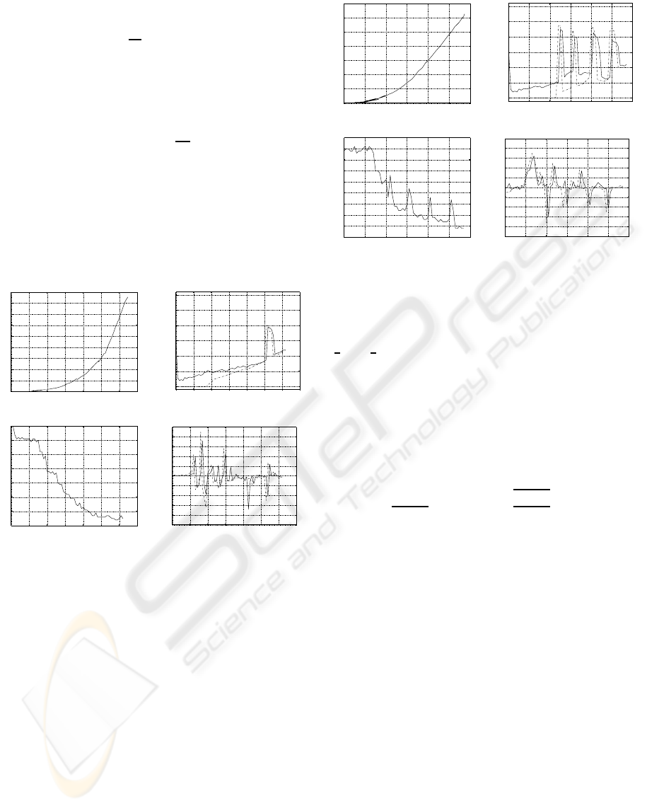
The results are illustrated in Fig. 3, 4. This method
is good at controlling x,y,θ to zeros. However, in ex-
periment 1 the car moved away from the garage to the
position (46,77) before backing into the garage. This
causes a safety problem. The phenomenon happens
because the driving velocity is determined automati-
cally and it can not be predicted where the car will
make a turn. In this sense this method cannot be ap-
plied to parking control when the initial orientation
angle is large.
0 10 20 30 40 50
0
10
20
30
40
50
60
70
80
x[cm]
y[cm]
(a) x− y path
0 5 10 15 20 25 30 35
−15
−10
−5
0
5
10
15
time[s]
Velocity[cm/s]
(b) Driving velocity
0 5 10 15 20 25 30 35
0
10
20
30
40
50
60
70
80
90
time[s]
Orientation Angle[deg]
(c) Orientation angle
0 5 10 15 20 25 30 35
−50
−40
−30
−20
−10
0
10
20
30
40
50
time[s]
Steering Angle[deg]
(d) Steering angle
Figure 3: Khennouf-Wit method: Experiment 1.
0 10 20 30 40 50
0
2
4
6
8
10
12
14
16
18
x[cm]
y[cm]
(a) x− y path
0 2 4 6 8 10
−15
−10
−5
0
5
10
15
time[s]
Velocity[cm/s]
(b) Driving velocity
0 2 4 6 8 10
0
5
10
15
20
25
30
35
time[s]
Orientation Angle[deg]
(c) Orientation angle
0 2 4 6 8 10
−50
−40
−30
−20
−10
0
10
20
30
40
50
time[s]
Steering Angle[deg]
(d) Steering angle
Figure 4: Khennouf-Wit method: Experiment 2.
AN EXPERIMENTAL COMPARISON OF NONHOLONOMIC CONTROL METHODS
209
4 ASTOLFI’S METHOD
This approach is proposed by Astolfi(Astolfi, 2000).
First, the next coordinate transformation (σ-process)
y
1
= z
0
, y
2
= z
2
, y
3
= z
1
/z
0
(10)
is introduced to make the chained system (6) discon-
tinuous. The transformed system is
˙y
1
= v
0
, ˙y
2
= v
1
, ˙y
3
=
y
2
− y
3
y
1
v
0
. (11)
When
v
0
= −ky
1
, k > 0 (12)
is applied, y
1
is stabilized and
˙y
2
˙y
3
=
0 0
−k k
y
2
y
3
+
1
0
v
1
(13)
is controllable. Hence, a linear feedback
v
1
= − f
2
y
2
+ f
3
y
3
, f
2
> k, f
3
> f
2
(14)
can stabilize y
2
, y
3
. As a result, the original states
z
1
,z
2
,z
3
are also stabilized.
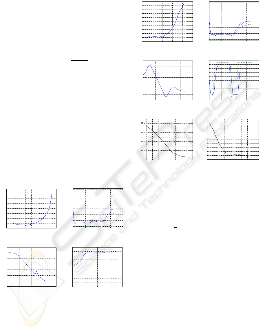
The responses are shown in Figs. 5 and 6. As is
seen from the measured data, the (x,y) path is pretty
smooth, but the steering angle does not converge to
zero. Further, the y coordinate moves to the oppo-
site side when the initial orientation angle θ is over
80[deg] (Fig. 5), which may cause a safety problem.
0 5 10 15 20 25 30 35 40
−15
−10
−5
0
5
10
15
20
25
y[cm]
(a) x− y path
0 5 10 15 20
−15
−10
−5
0
5
10
15
time[s]
Velocity[cm/s]
(b) Driving velocity
0 5 10 15 20
−40
−20
0
20
40
60
80
100
time[s]
Orientation Angle[deg]
(c) Orientation angle
0 5 10 15 20
−50
−40
−30
−20
−10
0
10
20
30
40
50
time[s]
Steering Angle[deg]
(d) Steering angle
Figure 5: Astolfi’s method: Experiment 1.
5 SORDALEN-EGELAND
METHOD
Sordalen-Egeland method uses a periodic v
0
to drive
the car and during this motion a time-varying v
1
(t) is
applied to attenuate z
1
,z
2
exponentially.
0 10 20 30 40 50
−2
0
2
4
6
8
10
12
14
16
18
y[cm]
(a) x− y path
0 5 10 15 20
−15
−10
−5
0
5
10
15
time[s]
Velocity[cm/s]
(b) Driving velocity
0 5 10 15 20
−10
0
10
20
30
40
50
60
time[s]
Orientation Angle[deg]
(c) Orientation angle
0 5 10 15 20
−50
−40
−30
−20
−10
0
10
20
30
40
50
time[s]
Steering Angle[deg]
(d) Steering angle
0 2 4 6 8 10 12 14 16 18
0
5
10
15
20
25
30
35
40
45
time[s]
x[cm]
(c) x coordinate
0 2 4 6 8 10 12 14 16 18
−2
0
2
4
6
8
10
12
14
16
18
time[s]
y[cm]
(d) y coordinate
Figure 6: Astolfi’s method: Experiment 2.
The control law is as follows: let the period be T
and Z
2
= (z
1
,z
2
)
T
, set v
0
(t) in iT ≤ t < (i+ 1)T as
v
0
(t) = k(z(iT)) f(t) (15)
in which f(t) =
1
2
(1−cos2πt/T), G(Z
2
) = ckZ
2
k
1/2
2
,
k(z(iT)) = sat(−[z
0
(iT) + G(Z
2
)sgn(z
0
(iT))]β, K).
Here β > 0 ,K > 0 ,c > 0 are design parameters and
sat(x,K) is a saturation function of x with peak value
K. On the other hand, in iT ≤ t < (i + 1)T v
1
(t) is
determined as 0 when z
0
(iT) = 0, and
v
1
(t) = [γ
2
,γ
3
]Z
2
, (z
0
(iT) 6= 0) (16)
where γ
2
= −λ − f
3
(t)λ, γ
3
= [−λ
2
f(t) −
2λ
˙
f(t)] f(t)/k(z(iT)) and λ > 0 is a parameter.
The results are shown in Fig. 7. The experiment
failed when the initial orientation angle θ is around
80[deg] because the car moves out of the sensing
range of PSD camera with an approximately 0[deg]
steering angle. Moreover, the tuning of parameter is
rather difficult since there are many parameters in the
control law. The oscillation in response in intrinsic to
this method. So this method is not suitable for parking
control.
ICINCO 2009 - 6th International Conference on Informatics in Control, Automation and Robotics
210
0 10 20 30 40 50
0
2
4
6
8
10
12
14
16
18
x[cm]
y[cm]
(a) x− y path
0 2 4 6 8 10 12
−15
−10
−5
0
5
10
15
time[s]
Velocity[cm/s]
(b) Driving velocity
0 2 4 6 8 10 12
0
5
10
15
20
25
30
35
time[s]
Orientation Angle[deg]
(c) Orientation angle
0 2 4 6 8 10 12
−50
−40
−30
−20
−10
0
10
20
30
40
50
time[s]
Steering Angle[deg]
(d) Steering angle
Figure 7: Sordalen-Egeland method: Experiment 2.
6 IKEDA-NAM-MITA METHOD
The control procedure of this method is divided into
two steps. In step 1, the input is determined as
v
0
= −λ
2
z
1
z
2
, v
1
= −λ
1
z
2
, λ
2
> λ
1
. (17)
Then the closed loop system becomes
˙z
0
= −λ
2
z
1
z
2
, ˙z
1
= −λ
2
z
1
, ˙z
2
= −λ
1
z
2
(18)
and (z
2
,z
1
) → 0. Note that z
1
/z
2
is bounded if λ
2
>
λ
1
. In step 2, the input is switched to
v
0
= −λ
3
z
0
, v
1
= −λ
1
z
2
(19)
once z
2
is sufficiently close to zero. The correspond-
ing closed loop system changes to
˙z
0
= −λ
3
z
0
, ˙z
1
= −λ
3
z
0
z
2
, ˙z
2
= −λ
1
z
2
(20)
and (z
0
,z
2
) → 0. In this process z
1
will not deviate
far away from 0 because the initial values of z
1
,z
2
are
sufficient small due to the control in step 1. In the
experiment, the input is switched back to step 1 if z
2
deviates far away from zero due to disturbance.
In the experiments, the input of step 1 is used if
|θ| ≤ 0.1[rad]. Otherwise the input of step 2 is used.
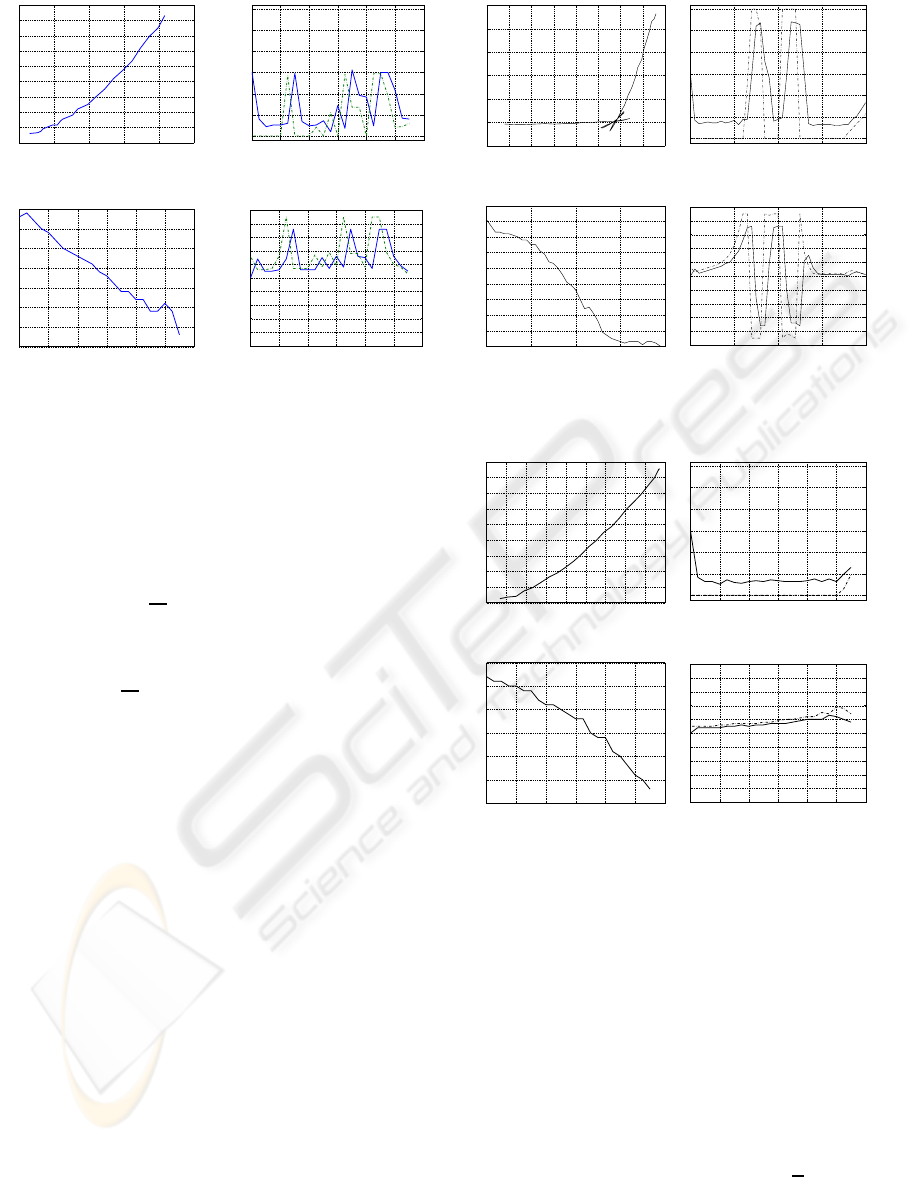
As can be seen from Fig.8 and 9, this method is
able to control x,y, θ to zeros pretty good. But in the
first experiment, the car moves back and forth four
times around the x axis. However, compared with
Khennouf-Wit Method the change of the direction of
the driving velocity occurs only in positions that are
far away from the origin, it is not so severe a draw-
back.
0 5 10 15 20 25 30 35 40
−5
0
5
10
15
20
25
x[cm]
y[cm]
(a) x− y trajectory
0 5 10 15 20
−15
−10
−5
0
5
10
15
time[s]
Velocity[cm/s]
(b) Driving velocity
0 5 10 15 20
0
10
20
30
40
50
60
70
80
90
time[s]
Orientation Angle[deg]
(c) Orientation angle
0 5 10 15 20
−50
−40
−30
−20
−10
0
10
20
30
40
50
time[s]
Steering Angle[deg]
(d) Steering angle
Figure 8: Ikeda-Nam-Mita method: Experiment 1.
0 5 10 15 20 25 30 35 40 45
0
2
4
6
8
10
12
14
16
18
x[cm]
y[cm]
(a) x− y trajectory
0 2 4 6 8 10 12
−15
−10
−5
0
5
10
15
time[s]
Velocity[cm/s]
(b) Driving velocity
0 2 4 6 8 10 12
5
10
15
20
25
30
35
time[s]
Orientation Angle[deg]
(c) Orientation angle
0 2 4 6 8 10 12
−50
−40
−30
−20
−10
0
10
20
30
40
50
time[s]
Steering Angle[deg]
(d) Steering angle
Figure 9: Ikeda-Nam-Mita method: Experiment 2.
7 JIANG’S METHOD
In (Jiang, 2000) Jiang Proposed a robust exponential
regulation method for a class of nonholonomic sys-
tems with uncertainty.
First, a rotation of (x,y) coordinate is introduced
to avoid singularity in the transformation to canonical
form
x
0
= θ, x
1
= xsinθ− ycosθ
x
2
= xcosθ+ ysinθ, u
0
= u
1
1
L
tanφ. (21)
This transformation brings (1) into
˙x
0
= u
0
, ˙x
1
= x
2
u
0
, ˙x
2
= u− x
1
u
0
. (22)
AN EXPERIMENTAL COMPARISON OF NONHOLONOMIC CONTROL METHODS
211
Further, a state scaling
z
1
=
x
1
x
0
, z
2
= x
2
(23)
is introduced. Then based on backstepping, the fol-
lowing control input are obtained:
u
0
= −λ
0
x
0
(24)
u
1
= −[λ
2
+ λ
0
(λ
1
+ 1) +
λ
0
4
(x
2
0
− 1+ λ
1
+ λ
2
1
)]
×(z
2
− (λ
1
+ 1)z
1
), λ
0
, λ
2
> 0, λ
1
> 1.
It is clear from the Figs. Please place \label
after \caption and Please place \label after
\caption that the car moves back and forth near
the garage which may cause safety problem. Also,
the steering angle is quite oscillatory and so is the ori-
entation angle as its consequence.
0 10 20 30 40 50 60 70
0
5
10
15
20
25
30
35
40
45
x[cm]
y[cm]
(a) x− y trajectory
0 5 10 15 20 25 30 35
−15
−10
−5
0
5
10
15
time[s]
Velocity[cm/s]
(b) Driving velocity
0 5 10 15 20 25 30 35
0
10
20
30
40
50
60
70
time[s]
Orientation Angle[deg]
(c) Orientation angle
0 5 10 15 20 25 30 35
−50
−40
−30
−20
−10
0
10
20
30
40
50
time[s]
Steering Angle[deg]
(d) Steering angle
Figure 10: Experiment 1(x(0)=64.7[cm], y(0)=42.8[cm],
θ(0)=70[deg]).
8 LIU-SAMPEI METHOD
This method(Liu et al., 2006) evolved from Sampei’s
method(Sampei and et al., 1995). Its essence is to at-
tenuate the orientation angle θ and y coordinate while
drive the car back and forth on the allowed road, then
finally park the car into the garage. A distinguishing
feature of this method is that the driving velocity can
be determined freely.
Let z
∗
2
be
z
∗
2
= −C
1
sgn(v
0
)z
1
, C
1
> 0 (25)
and determine the control input v
1
as
v
1
= −C
1
z
2
|v
0
| − z
1
v
0
−C
2
(z
2
− z
∗
2
)|v
0
|. (26)
0 10 20 30 40 50 60
0
5
10
15
20
25
30
35
x[cm]
y[cm]
(a) x− y trajectory
0 5 10 15 20 25 30
−15
−10
−5
0
5
10
15
time[s]
Velocity[cm/s]
(b) Driving velocity
0 5 10 15 20 25 30
0
5
10
15
20
25
30
35
40
45
time[s]
Orientation Angle[deg]
(c) Orientation angle
0 5 10 15 20 25 30
−50
−40
−30
−20
−10
0
10
20
30
40
50
time[s]
Steering Angle[deg]
(d) Steering angle
Figure 11: Experiment 2(x(0)=57.3[cm], y(0)=31.4[cm],
θ(0)=39[deg]).
Then the derivative of Lyapunov function V =
1
2
z
2
1
+
1
2
(z
2
− z
∗
2
)
2
satisfies
˙
V = −C
1
z
2
1
|v
0
| − C
2
(z
2
−
z
∗
2
)
2
|v
0
| which is negative semidefinite. Hence, the
convergence of (z
1
,z
2
) is guaranteed.
The input v
0
is selected as follows: (1) Take v
0
arbitrarily if z
2
1
+(z
2
−z
∗
2
)
2
> γ. (2) v
0
= −sgn(z
0
)|U|
when z
2
1
+ (z
2
− z
∗
2
)
2
< γ so as to stabilize z
0
. Here,
U is given by
U =
u
max
βcos(θ) if
p
x
2
+ y
2
≥ βu
max
p
x
2
+ y
2
βcos(θ) if
p
x
2
+ y
2
< βu
max
(27)
u
max
is the maximum of driving velocity and β is
a deceleration factor.
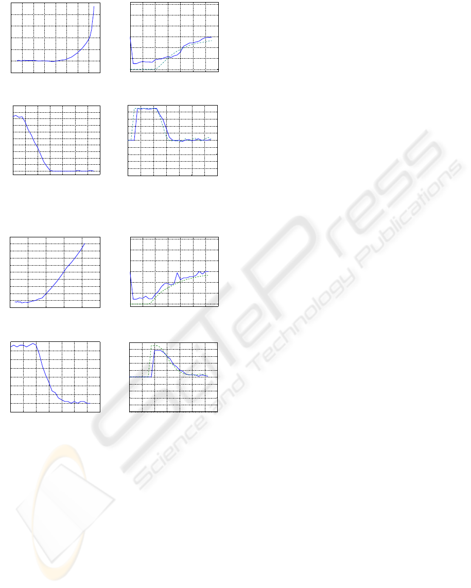
The experiment data are illustrated in Fig. 12, 13.
This method can stabilize x,y,θ from any initial state
and provides the best performance for parking con-
trol.
9 CONCLUDING REMARKS
The applicability of 6 typical control methods for
chained system has been tested experimentally by us-
ing an automatic parking benchmark. The results in-
dicate that Astolfi’s method(Astolfi, 2000) and Ikeda-
Nam-Mita method(Ikeda et al., 2000) may be ap-
plied to parking control when the initial orientation
angle is not too big. It is noted that in Astolfi’s
method the steering angle does not converge to zero.
Liu(Liu et al., 2006)-Sampei(Sampei and et al., 1995)
method is applicable to any situations. Meanwhile,
Khennouf-Wit method and Jiang’s method should be
ICINCO 2009 - 6th International Conference on Informatics in Control, Automation and Robotics
212
0 5 10 15 20 25 30 35 40
−5
0
5
10
15
20
25
x[cm]
y[cm]
(a) x− y path
0 2 4 6 8 10 12 14
−15
−10
−5
0
5
10
15
time[s]
Velocity[cm/s]
(b) Driving velocity
0 2 4 6 8 10 12 14
0
10
20
30
40
50
60
70
80
90
100
time[s]
Orientation Angle[deg]
(c) Orientation angle
0 2 4 6 8 10 12 14
−50
−40
−30
−20
−10
0
10
20
30
40
50
time[s]
Steering Angle[deg]
(d) Steering angle
Figure 12: Liu-Sampei method: Experiment 1.
0 10 20 30 40 50
−2
0
2
4
6
8
10
12
14
16
18
y[cm]
(a) x− y path
0 2 4 6 8 10 12 14
−15
−10
−5
0
5
10
15
time[s]
Velocity[cm/s]
(b) Driving velocity
0 2 4 6 8 10 12 14
−5
0
5
10
15
20
25
30
35
time[s]
Orientation Angle[deg]
(c) Orientation angle
0 2 4 6 8 10 12 14
−50
−40
−30
−20
−10
0
10
20
30
40
50
time[s]
Steering Angle[deg]
(d) Steering angle
Figure 13: Liu-Sampei method: Experiment 2.
used with care due to safety concern. Sordalen-
Egeland method is not suitable for parking control un-
der steering angle and parking space limitation.
It is also worth noting that all methods, except
Liu-Sampei and Ikeda-Nam-Mita methods, guaran-
tees asymptotic stability, but their performances are
not as good as those of Liu-Sampei and Ikeda-Nam-
Mita methods. The author feels that the degrading of
performance is caused by killing the freedom of con-
trol (the driving velocity) in order to prove the asymp-
totic stability. In contrast, both Liu-Sampei method
and Ikeda-Nam-Mita method use switching of con-
trol input which provides the control flexibility and
leads to better performance, although it is very dif-
ficult to show their asymptotic stability. The author
strongly believe that control design based on asymp-
totic/exponential stability point of view is not suitable
for this class of control problems, the emphasis should
be put on improving the performance instead.
REFERENCES
Astolfi, A. (2000). Discountinuous control of non-
holonomic systems. Systems and Control Letters,
27(1):37–45.
H.Khennouf and Wit, C. (1996). Quasi-continuous expo-
nential stabilizers for nonholonomic system. Proc. of
13th IFAC World Congress, 2b(174):49–54.
Ikeda, T., Nam, T.-K., and Mita, T. (2000). Nonholonomic
variable constraint control of free flying robotics and
its convergence (in japanese). Journ. of Robotics So-
ciety of Japan, 18.
Jiang, Z.-P. (2000). Robust exponential regulation of non-
holonomic systems with uncertainties. Automatica,
pages 189–209.
Liu, K.-Z., Dao, M.-Q., and Inoue, T. (2006). An exponen-
tial ε-convergent control algorithm for chained sys-
tems and its application to automatic parking. IEEE
Trans. on Control Systems Technology, 14(6):1113–
1126.
Sampei, M. and et al. (1995). Arbitrary path tracking con-
trol of articulated vehicles using nonlinear control the-
ory. IEEE Trans. on Control Systems Technology,
3(1):125–131.
Sordalen, O. and Egeland, O. (1995). Exponential stabiliza-
tion of nonholonomic chained systems. IEEE Trans.
Automat. Control, 40:35–49.
AN EXPERIMENTAL COMPARISON OF NONHOLONOMIC CONTROL METHODS
213
