MODEL-BASED DESIGN OF CODE FOR PLC CONTROLLERS
Krzysztof Sacha
Warsaw University of Technology, Nowowiejska 15/19, 00-665 Warszawa, Poland
Keywords: Automatic program generation, Model verification, Finite state machine, Programmable logic controller.
Abstract: This paper describes a method for model-based development of software for programmable logic controllers
(PLC). The method includes modeling of a control algorithm, verifying the algorithm with respect to the
requirements, and automatically generating the code in one of the IEC 61131 languages. The modeling
language is UML state machine diagram, and the verification tool is UPPAAL model-checking toolbox. The
method has good scalability with respect to the number of the modeled objects and the ability to cope with
integer values by means of variables and function blocks.
1 INTRODUCTION
This paper describes a method for model-based
development of software for programmable logic
controllers – PLC. The method includes modeling of
a control algorithm, verifying the algorithm, and
automatically generating the code for a PLC.
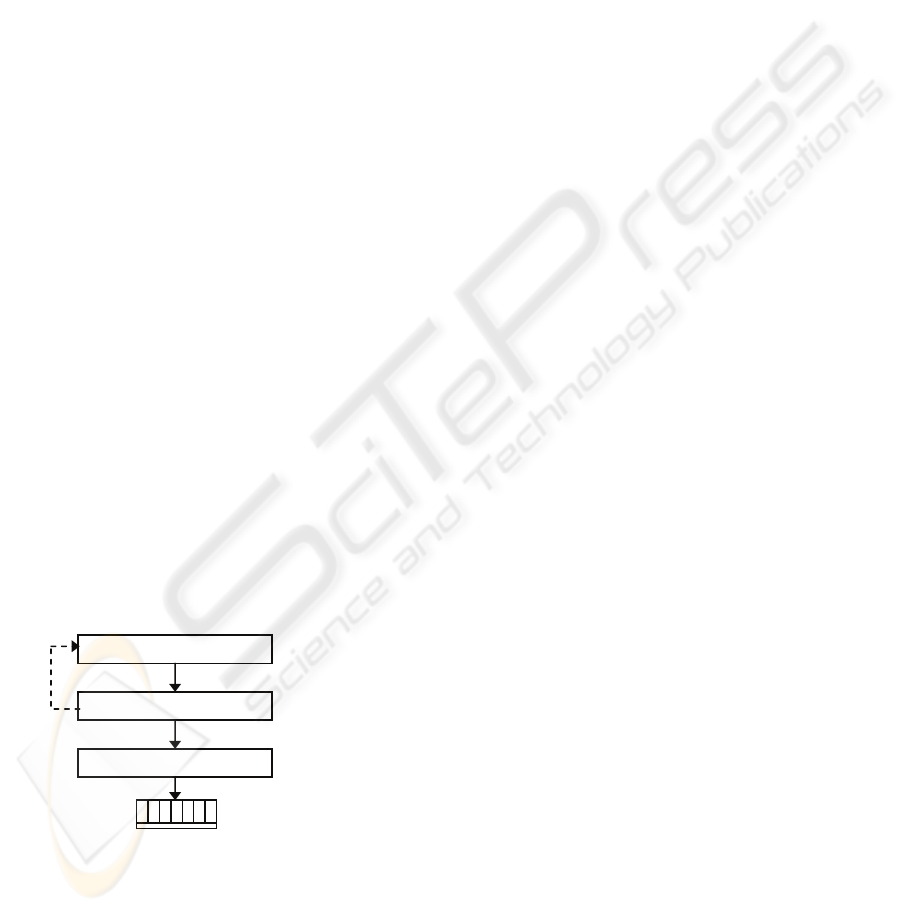
The development cycle is shown in Figure 1. The
modeling language is UML state machine diagram
(OMG, 2005), which has been widely accepted as a
means for specifying the controller at a suitable high
level of abstraction. The verification tool is the
UPPAAL model-checker (Behrmann et al, 2004).
When the verification has been finished, the
implementation code can be generated automatically
in one of the IEC 61131 languages (IEC, 1993).
Figure 1: Modeling, verification and implementation of
the program code.
A formal semantics for a UML state machine is
given by a translatable finite state time machine –
FSTM (Sacha, 2007, 2008). Modeling a controller in
UML, modeling the environment in UPPAAL, and
formulating safety requirements in a formal
language of CTL formulae are done manually. The
tasks of converting the model from UML to
UPPAAL and to FSTM, verifying the model, and
generating the program code are done automatically.
The unique features of the method described in
this paper are the use of UML state machine as a
problem modeling tool, and the ability to verify time
dependent behavior of the controller. Widely
accepted models of timed automata (Alur, Dill,
1996) and timed I/O automata (Kaynar et al, 2006)
are used mainly for modeling and verification of
time-dependent behavior of state systems. Still
another models of time triggered automata (Krcal et
al, 2004) and PLC-automata (Dierks, 1997) are used
for code generation only.
The paper is organized as follows. Section 2
gives an overview of PLC controller and finite state
time machine. Section 3 defines the semantics of
UML state machine in FSTM. Section 4 presents a
conversion algorithm from FSTM to UPPAAL and
explains the verification process. The conversion of
finite state time machine into a program code is
described in Section 5. A discussion of the results
and plans for future work are given in Conclusions.
2 PLC CONTROLLER
PLC is a computerized device that cooperates with
its environment through a set of input and output
signals. The controller executes in a loop, polling the
inputs and computing the values of the outputs.
Modelin
g
in UML
Verification in UPPAAL
automatic translation
automatic translation
Code
g
eneration in FSTM
compilation (STEP7)
PLC
Controlle
r
130
Sacha K. (2009).
MODEL-BASED DESIGN OF CODE FOR PLC CONTROLLERS.
In Proceedings of the 6th International Conference on Informatics in Control, Automation and Robotics - Signal Processing, Systems Modeling and
Control, pages 130-135
DOI: 10.5220/0002209801300135
Copyright
c
 SciTePress

The controller counts time using timers. A timer
can be activated in a given a set of states. An active
timer counts time and expires when it has continued
to be active for a predefined period of time. An
expired timer is perceived by the controller similarly
as an input signal. The execution of a controller can
be described in a pseudo-code, which creates a
reference model for PLC execution:
state = initial_state();
loop_forever {
input = poll_the_input();
timers =
set_timers(active_timers(state));
state = next_state(state,timers,input);
output = count_output(state);
set_the_output(output);
}
Board software of a PLC sets the initial state
(
initial_state), executes the loop (loop_
forever
), polls the input signals (poll_the_
input
) counts time and sets the expired timers
(
set_timers), and sets the output signals (set_
the_output). The programmer must only write a
code for selecting active timers (
active_timers),
and calculating the next state of the controller
(
next_state) and of the output (count_output).
The semantics of a PLC program is defined by a
finite state time machine (Sacha, 2007), which is a
tuple A
= ( S, Σ , Γ , τ , δ , s
0
, Ω , ω ) where
S is a finite set of states,
Σ is a finite set of input symbols,
Ω is a finite set of output symbols,
Γ is a finite set of variables called timer symbols,
τ : Γ → 2
S
× N
+
is an injective function, called
timer function (with two projections
τ
S
: Γ → 2
S
and
τ
N
: Γ → N
+
, respectively),
δ : S × Σ × 2
Γ
→ S is a partial function, called
transition function, such that:
[(
s, a, T ) ∈ Dom( δ )] ⇔ ( ∀ t ∈ T )[ s ∈ τ
S
( t )]
s
0
∈ S is the initial state,
ω : S → Ω is an output function.
Notation: N
+
is the set of positive integers, Dom( δ )
is the domain of a function
δ , card(X) is the
cardinality of a set X, and
φ is an empty set.
Finite state time machine looks much like a
Moore automaton with three additional elements:
Γ ,
τ , ε , which add to the model the dimension of time.
A timer symbol t
∈Γ is a variable, which takes values
from the set N
+
. The current value of t is interpreted
as the duration of a period of time. Timer function
τ
assigns to each timer a group of states and a constant
value. The meaning is such that timer t is enabled,
i.e. counts time, as long as the automaton resides in
one of the states from
τ
S
( t ) and it expires when the
current value of t exceeds
τ
N
( t ).
Timer symbols in
Γ can be set in an arbitrary
order and denoted t
1
... t
n
. The valuation ŧ of timer
symbols can be described as a vector of values ŧ. The
current value of a timer t
i
is denoted ŧ
i
.
The execution of a finite state time machine
starts in state s
0
with the values of all timers equal to
0. For a given state s
k
and a valuation of timers ŧ
k
there exists a set of expired timers, defined as:
Θ ( s
k
, ŧ
k
) = { t
i
∈Γ : s
k
∈τ
S
( t
i
) and ŧ
i
k
≥ τ
N
(t
i
) }
The machine executes in a state (
s
k
, ŧ
k
) by taking
an input symbol a
k
and moving to the next state s
k + 1
defined by the transition function:
s
k + 1
=δ (s
k
,a
k
, Θ ( s
k
, ŧ
k
) ) where k = 0,1,.....
When the machine enters a state s
k + 1
time
advances and the values of timers change reflecting
the elapsed time interval:
ŧ
i
k
+ 1
=
When the valuation of timers ŧ changes, the set
Θ
of expired timers may change as well. This way a
finite state time machine can respond to the flow of
time, even if s
k + 1
= s
k
and a
k + 1
= a
k
. Please note that
the last argument of
δ is a set of expired timers,
hence, no conflict exists if several timers expire at
the same time instant.
The state space of a PLC as well as of an FSTM
can be defined by enumerating all of the elements,
eg. S
= { s
1
, s
2
,..., s
n
}. An alternative way is to allow
for using variables and to define the state space as a
Cartesian product of a set of enumerated elements
and a set of all possible valuations of those
variables. This is only a shorthand notation, which
does not add any new semantics to the model, and
therefore it is not shown in the formal definition.
In the rest of this paper, we will adopt a naming
convention of UPPAAL (Behrmann et al, 2004) and
refer to the enumerated elements of state as
locations. Locations will be shown in graphical
models explicitly, as the nodes of a graph, while
variables will be referred to by guard expressions
and will be assigned values within actions of
transitions.
⎧
⎨
ŧ
i
k
+
1if
s
k + 1
∈
τ
S
(
t
i
) and
s
k
∈
τ
S
(
t
i
)
0 otherwise
⎩
MODEL-BASED DESIGN OF CODE FOR PLC CONTROLLERS
131

3 UML STATE MACHINE
UML state machine diagram is a graph composed
of nodes, which are locations, and edges, which are
labeled transitions. A transition can be triggered by a
signal received from the outside. A transition which
is triggered can fire, if the corresponding guard
expression over a set of variables evaluates to true.
Firing of a transition can move the machine to a new
location, change the values of variables and send a
signal. This way, the state space of a UML state
machine is a Cartesian product of the set of locations
and the set of all possible valuations of variables.
UML allows for nesting of locations. However, a
hierarchy of locations can always be flattened. A
formal model and an algorithm for flattening the
hierarchy were described in detail in (Sacha, 2007)
an will not be discussed in the rest of this paper.
Relating this model to a PLC, one can note that a
received signal corresponds to a combination of the
input signals of the PLC, and a sent signal
corresponds to a combination of the output signals.
States of an UML state machine and transitions
between states correspond to states of a PLC and to
the next-state function defined by a program code.
A conversion algorithm of a UML state machine
into a FSTM can be described as follows.
S equals to the Cartesian product of the set of all
locations of the UML state machine and the
valuations of variables used in guard expressions.
Σ equals to the set of external signals, which trigger
transitions in the UML state machine; a signal is a
combination of all the input signals of the PLC.
Γ is a set of timer symbols t
1
,...,t
n
; there is one timer
symbol t
i
for each timed transition (i.e. transition
with an after clause) in the UML state machine,
τ is the timer function, which assigns to each timer
symbol t
i
created for a timed transition T a pair
composed of a source state of this transition and
the value of the after clause of this transition.
δ is the transition function δ : S × Σ × 2
Γ
→ S , such
that:
δ ( s
1
, a, T ) = s
2
if and only if there exists a
transition in the UML state machine diagram such
that s
1
is the source and s
2
the destination state of
this transition, and either a is the event that
triggers this transition (in this case T
= φ ), or
T
= {t
i
} and t
i
is the timer symbol of this timed
transition (ie.
δ ( s
1
, a, T ) = s
2
for all a ∈Σ ).
s
o
is the initial state of the UML state machine.
Ω equals to the set of combinations of all the output
signals of the PLC that are set by the actions of
the UML state machine.
ω is the output function, which assigns to each state
s
∈ S the output symbol q ∈Ω , which is set by all
transitions to s.
Example. Consider a railroad crossing controlled by
a PLC. There are a number of railway tracks within
the crossing, and a number of trains can approach
the crossing simultaneously (one train on a track is
allowed). The movement of trains is controlled by a
set of semaphores that can prevent trains from
entering the crossing. The road traffic is controlled
by a gate that can be open or closed. A semaphore
can be operated by a controller to display green
light, when a train approaches, but not earlier than
after the gate has been closed. Opening and closing
states of the gate are confirmed to the controller by
the input signals: up and down, respectively. Closing
the gate must last less than 30 seconds, or else an
alarm must sound. The semaphores are red and the
gate is up in the initial state of the crossing.
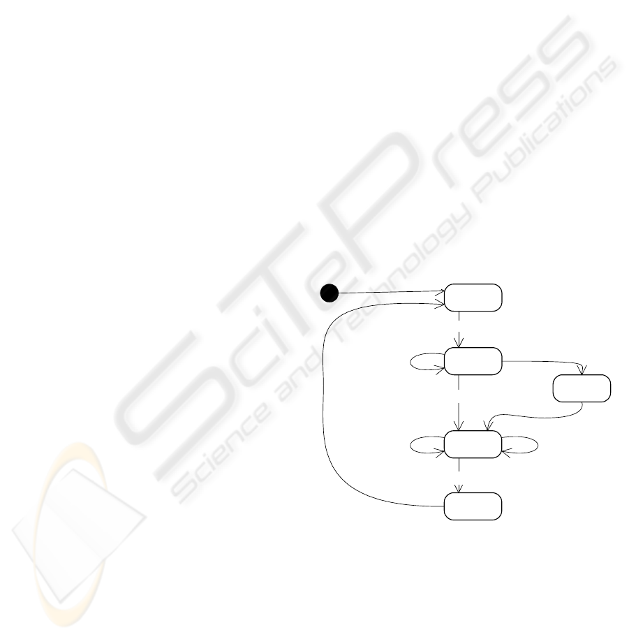
An algorithm for the railroad crossing controller
is shown in Figure 2. The locations within the graph
correspond to states of the crossing with respect to
train positions. The transitions bear labels of the type
event / action, where event corresponds to a
condition on the input signals or timers, and action
corresponds to setting the values of variables.
Outside
Entering
Inside
approach(i) / a(i):=1,close
approach(i) / a(i):=1
down / MOV(a,green)
Leaving
when: a==0 / MOV(0,green),open
Alarm
after: 30 / sound
down / MOV(a,green)
leave(i) / a(i):=0
approach(i) /
a(i):=1, green(i)
up
/ MOV(0,green),open
Figure 2: UML model of the railroad crossing controller.
The positions of particular trains are signaled to
the controller by short input pulses approach(i) and
leave(i), i=0,...n-1. The appearance of an approach-
pulse is stored in a vector variable a(i), i=0,...n-1
and makes the controller to close the gate. When the
gate is down, the controller uses the stored data to
send green signals to the appropriate semaphores –
the function MOV(a,green) sends a green-signal for
each train, which approaches the crossing.
ICINCO 2009 - 6th International Conference on Informatics in Control, Automation and Robotics
132

The controller keeps track of all the trains inside
the crossing, and waits until the last train has left. If
this is the case, the controller turns the green signals
off, opens the gate and waits until the gate is up.
Vector a is part of the controller state. This way,
there are in fact as many Entering and Inside states
as are the combinations of values in vector a. Output
signals of the state machine are open and close to
operate the gate, and the signals green(i) to operate
the semaphores to display green or red.
FSTM model of the controller has the same set
of locations and the same set of variables. It has a
single timer symbol t, and the timer function
τ
S
( t ) = {Entering} and τ
N
( t ) = 30. The transition
function is defined by the set of all the transitions of
the UML state machine. The sets of input and output
symbols are the combinations of input and output
signals.
4 VERIFICATION
UPPAAL is a toolbox for modeling and verification
of real time systems, based on the theory of timed
automata. The core part of the toolbox is a model-
checking engine, which enables for verification of
properties defined as CTL path formulae.
A timed automaton (Alur, Dill, 1996), as used in
UPPAAL, is a finite state machine extended with
clock variables that evaluate to positive real numbers
and state variables that evaluate to discrete values.
State variables are part of the state. All the clock
variables progress simultaneously. An automaton
may fire a transition in response to an action, which
can be thought of as an input symbol, or to a time
action related to the expiration of a clock condition.
A clock variable can be reset to zero at a transition.
A set of timed automata can be composed into a
network over a common sets of clocks, variables and
actions. This way a cooperation between a controller
and a controlled plant can be modeled.
The use of a dense-time model-checker to verify
a discrete-time model may look as an overkill. But
in fact it is not, because the environment of the
controller works in real-time and must be modeled
using a dense-time method.
A conversion algorithm of FSTM into UPPAAL
is described in (Sacha, 2008).
Verification. UPPAAL can verify the model with
respect to the requirements, expressed formally as
CTL formulae. To do this, UPPAAL model-checker
evaluates path formulae over the reachability graph
of a network of timed automata.
The query language consists of state formulae
and path formulae. A state formula is an expression
that can be evaluated for a particular state in order to
check a property (e.g. a deadlock). Path formulae
quantify over paths of execution and ask whether a
given state formula
ϕ can be satisfied in any or all
the states along any or all the paths.
Path formulae can be classified into three types:
• Reachability properties: E<>
ϕ . (will ϕ be
satisfied in a state of a path?)
• Safety properties: E[]
ϕ and A[] ϕ . (will ϕ be
satisfied in all the states along a single or along
all paths?)
• Liveness properties: A<>
ϕ and ψ --> ϕ . (will ϕ
eventually be satisfied? will
ϕ respond to ψ ?)
Example. Consider again the railroad crossing
described in Section 3. A train cannot be stopped
instantly. When a train is detected by a train position
sensor, a controller has 30 seconds to close the gate
and display a green signal, which allows the train to
continue its course. After these 30 seconds, it takes
further 20 seconds to reach the crossing. Otherwise,
if the green signal is not displayed within these 30
seconds, the train must break in order to stop safely
before the crossing. Closing the gate must last less
than 20 seconds, or else an alarm must sound. The
gate can be opened when the position sensor has sent
a leave signal after the last train has left the crossing.
The environment of the controller consists of a
number of trains and a gate. Each of these elements
can be modeled in UPPAAL and synchronized with
the controller within a network of timed automata.
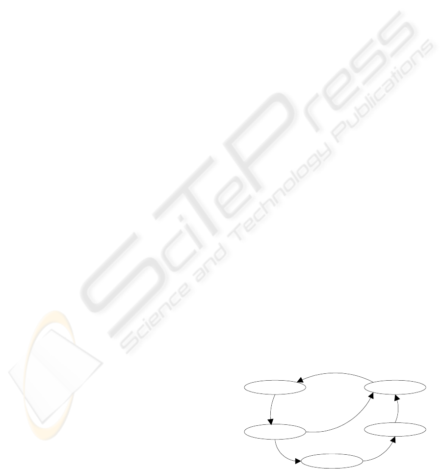
The template of a train is shown in Figure 3.
Actions, which names bear the suffix ‘?’, act like
input symbols that enable the associated transitions.
Actions, which names bear the suffix ‘!’, act like
output symbols that are passed to other automata in
order to trigger the respective input symbols. This
way the execution of one automaton can control the
execution of a other automata.
Faraway
Approaches
i:=id
approach!
t:=0
On crossing
i==id && t<=30
green?
t:=0
i:=id
leave!
t >20
Starting
Stop
t>=30
i==id
green?
t:=0
t >10
t:=0
t<=30
t<=25
t<=40
Figure 3: UPPAAL model of a train.
MODEL-BASED DESIGN OF CODE FOR PLC CONTROLLERS
133

Time invariant t
≤ 30 of state Approaches forces a
transition after 30 seconds have passed since the
train has entered the state. This models the necessity
of breaking the train if green has not been displayed
in time. Time condition t
> 20 at the transition from
On crossing to Faraway reflects the minimum time
of passing the crossing by a fast train. Time
invariant t
≤ 40 of the state On crossing reflects the
maximum time of passing by a slow train.
The template is parameterized with the train
identifier id. A set of n trains, e.g. four, can be
generated using the values of id
= 0 through 3.
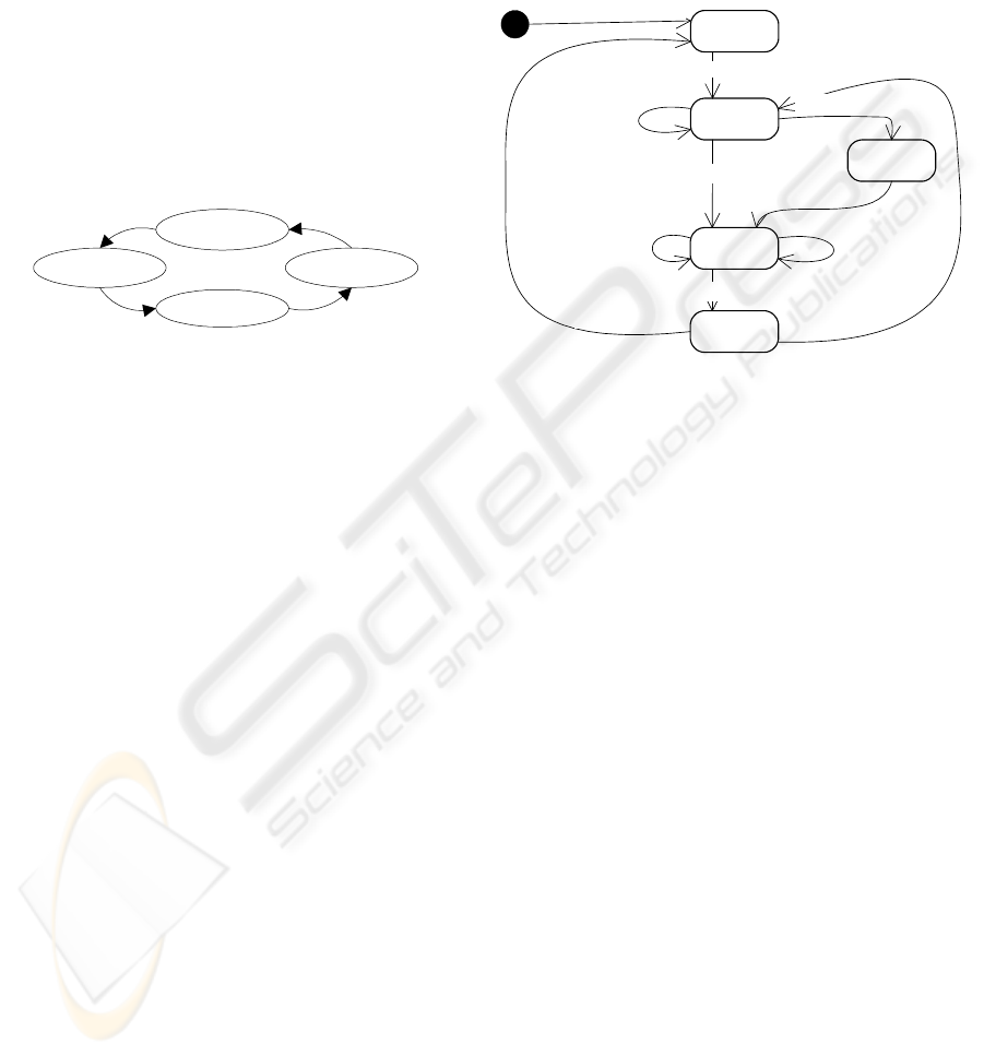
A model of the gate is shown in Figure 4. Time
invariants t
≤ 20 at states Closing and Opening reflect
time that it takes to close or to open the gate.
Open
Closed
OpeningClosing
down!
open?
close?
up!
t<=20 t<=20
Figure 4: UPPAAL model of the gate.
The simple reachability properties can check if a
given state is reachable:
• E<> train1.On crossing: This checks if train 1
can pass the crossing (a similar property can be
checked for other trains).
• E<> ( train1.On crossing && train2.On crossing
&& train3.On crossing && train4.On crossing ):
This checks if all the trains can move through the
crossing simultaneously.
The safety properties can check that unsafe states
will never happen:
• A [] ( train1.On crossing or train2.On crossing or
train3.On crossing or train4.On crossing ) imply
gate.Closed: This ensures that each time a train is
passing the crossing, the gate is closed.
• A [] ( gate.open imply (
¬ train1.On crossing &&
¬ train2.On crossing && ¬ train3.On crossing
&&
¬ train4.On crossing ) ): This ensures that
each time the gate is open, a train is not on the
crossing.
The liveness properties can check consequences
of an event, e.g.:
• train1.Approaches --> train1.On crossing: This
ensures that whenever train 1 approaches the
crossing, it will eventually pass it.
In our example the liveness condition is not
satisfied: Assume that the train 2 approaches when
train 1 is just leaving. The controller does not react
to approach in state Leaving, hence, the transition to
Outside appears without displaying green signal for
train 2. The train will stop and can never reach the
crossing.
The corrected finite state time machine model of
the controller is shown in Figure 5.
approach(i) /
a(i)=1,close
Outside
Entering
Inside
approach(i) / a(i):=1,close
approach(i) / a(i):=1
down / MOV(a,green)
Leaving
when: a==0 / MOV(0,green),open
Alarm
after: 30 / sound
down / MOV(a,green)
leave(i) / a(i):=0
approach(i) /
a(i):=1, green(i)
up
/ MOV(0,green),open
Figure 5: The corrected model of the controller.
5 CODE GENERATION
The semantics of a PLC program is defined within
the reference model by the semantics of its
programming language (IEC, 1993), e.g. ladder
diagram or structured text. The behavior of a finite
state time machine has been defined in Section 2. By
that means a method for translating a high level
abstract model of finite state time machine ( S,
Σ , Γ ,
τ , δ , s
0
, Ω , ω ) into a PLC program can formally be
defined in the following steps:
1. Mapping of sets
Σ , Ω into the input and output
signals of PLC. This can be an arbitrary one-to-
one mapping (coding of symbols).
2. Mapping of the set of locations which define part
of state S into the values of flip-flops. This can be
an arbitrary one-to-one mapping (coding of
states). Mapping of the variables which define the
other part of the state into the variables within the
memory of the PLC.
3. Mapping of set
Γ into the set of timers. A
separate timer with the expiration time equal to
τ
N
( t ) is allocated for each timer symbol t ∈ Γ .
4. Defining the function
active_timers
consistently with function
τ . This function defines
the input signals of all timer blocks. The input
signal of a timer block allocated for a timer t
∈ Γ ,
ICINCO 2009 - 6th International Conference on Informatics in Control, Automation and Robotics
134

is a Boolean function over the set of flip-flops
used for coding of states, such that it is true in
state s if and only if s
∈ τ
S
(t).
5. Defining function
next_state consistently with
function
δ . This function defines the set and reset
signals of flip-flops, which have been used for
coding of states. The signal to set (reset) a flip-
flop is a Boolean function over the set of flip-
flops, input signals of PLC and output signal of
timer blocks, such that it is true if and only if this
flip-flop is set (reset) in the next state of FSTM.
6. Defining function
count_output consistently
with function
ω . This function defines the values
of output signals of PLC. The value of an output
signal is a Boolean function over the set of flip-
flops, such that it is true if and only if this output
signal is set in the current state of FSTM.
Example. To capture four trains within the crossing,
we need four approach and four leave input signals
from trains, plus two up and down input signals from
the gate (Figure 5). There are four green signals
output to semaphores, two signals open and close to
the gate and a sound output signal. Any combination
of the input (output) signals corresponds to an input
(output) symbol. PLC controller stores the locations
as states of its internal flip-flops. At least three flip-
flops are needed. A selected coding for states and
output signals of the controller is shown in Table 1.
Table 1: The coding of states and output signals.
M1 M2 M3 a[i] State close open green(i) sound
0 0 0 0 Outside 0 0 0 0
0 1 0 a(i) Entering 1 0 0 0
1 1 0 a(i) Inside 0 0 a(i) 0
1 0 0 0 Leaving 0 1 0 0
0 1 1 a(i) Alarm 1 0 0 1
The program for PLC is a ladder diagram (IEC,
1993) consisting of a sequence of lines, each of
which describes a Boolean expression to set or reset
a flip-flop or an output signal, to activate a timer, or
to call a function block to operate a variable,
according to the values of input signals, states of
flip-flops, variables and timers. The expressions
reflect the coding of locations and implement the
functions
active_timers, next_state and
count_output described in Section 2. An example
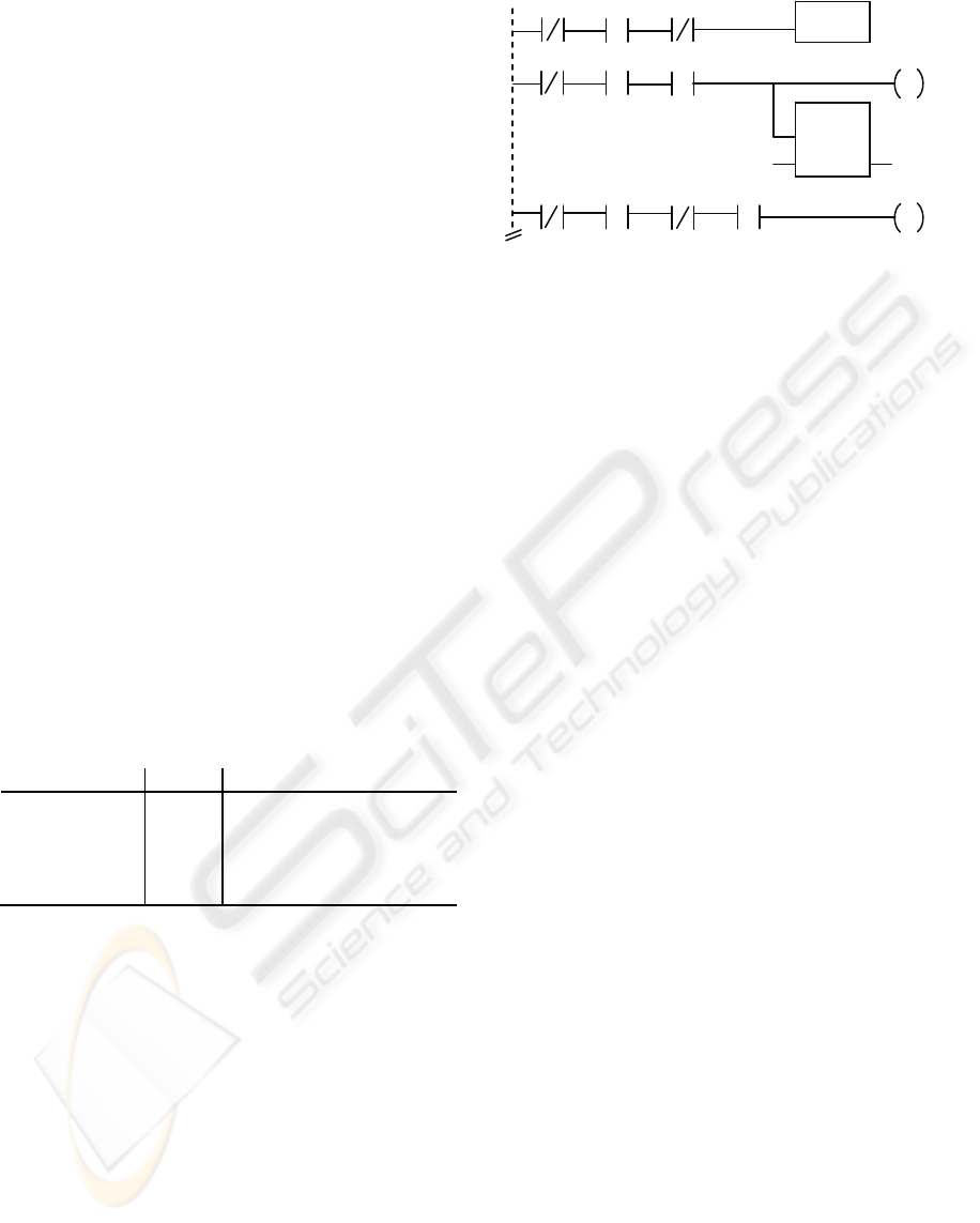
is shown in Figure 6, which presents the transitions
from Entering to Alarm and from Entering to Inside
(Figure 5). M11 and M13 are auxiliary flip-flops,
which mirror the main flip-flops M1 and M3, in
order to assure atomicity of the transitions.
Figure 6: A fragment of the ladder diagram program for
the railroad crossing controller.
6 CONCLUSIONS
A method is described for the specification,
verification and automatic generation of code for
PLC controllers. The advantages of the method are
intuitive modeling by means of a widely accepted
UML state machine, and a potential for automatic
verification and implementation of the model.
A tool which implements the steps of the method
has been implemented and verified on small scale
examples. The verification included experiments in a
lab equipped with a few process models and a set of
S7 PLC controllers from Siemens.
REFERENCES
Alur R., Dill D., 1996. Automata-theoretic verification of
real-time systems. In Formal Methods for Real-Time
Computing, Trends in Software Series, John Wiley.
Behrmann G., David A., Larsen K.G, 2004. A Tutorial on
Uppaal, Aalborg University.
Dierks, H., 1997. PLC-Automata: A New Class of
Implementable Real-Time Automata. LNCS 1231.
Springer, Berlin.
IEC, 1993. Programmable controllers – part 3:
Programming languages.
Kaynar D.K., Lynch N.A., Segala R., Vaandrager F.W.,
2006. The Theory of Timed I/O Automata. Synthesis
Lecture on Computer Science, Morgan & Claypool.
Krcal P., Mokrushin L., Thiagarajan P.S., Wang Yi. 2004.
Timed vs. Time Triggered Automata. LNCS 3170,
Springer-Verlag, Heidelberg.
OMG, 2005. Unified Modelling Language: Superstructure,
version 2.0.
Sacha K., 2007. Translatable Finite State Time Machine.
LNCS 4745, Springer, Berlin.
Sacha K., 2008. Model-Based Implementation of Real-
Time Systems. LNCS 5219, Springer, Berlin.
M1 M2
S
M
11
M2
TON
IN
M1
M3
down
M1 M2
S
M
13
M3
T
MOV_B
EN
IN
a
green
T
MODEL-BASED DESIGN OF CODE FOR PLC CONTROLLERS
135