
DYNAMICAL CLUSTERING TECHNIQUE TO ESTIMATE THE
PROBABILITY OF THE FAILURE OCCURRENCE
OF PROCESS SUBJECTED TO SLOW DEGRADATION
M. Traore, E. Duviella and S. Lecoeuche
Departement Informatique et Automatique, Ecole des Mines de Douai, France
Keywords:
Supervision, Pattern Recognition, Non-stationary data, AUDyC.
Abstract:
In this paper, we propose a supervision method which aims at determining pertinent indicators to optimize
predictive maintenance strategies. The supervision method, based on the AUto-adaptative and Dynamical
Clustering technique (AUDyC), consists in classifying in real time measured data into classes representative
of the operating modes of the process. This technique also allows the detection and the tracking of the slow
evolutions of the process modes. Based on the AUDyC technique, a method is proposed to estimate the
probabilities of the failure occurence of components in real time. This method is illustrated on the real case of
a temperature controller.
1 INTRODUCTION
Maintenance strategies consist in improving the
safety and the reliability of industrial processes, tak-
ing into account their characteristics and the cost of
maintenance plans (Grall et al., 2002). Amongst the
three principal types of maintenance strategies which
are proposed in the literature (Muller et al., 2004), i.e.
the corrective, the preventive and the predictive main-
tenance strategies, the predictive maintenance allows
the anticipation of failures and the optimal selection
of maintenance actions, by the estimation in real time
of the current state of the process components. This
strategy is generally based on supervision methods
and the estimation of the failure occurrence proba-
bilities of the components of the process. The ini-
tial selection of the components which are essential
to supervise, is performed by a dysfunctional anal-
ysis of the failure modes and their effects (FMEA:
Failure Mode and Effects Analysis). Then, the inter-
actions between each component are modelled by a
Fault Tree formalism (Lassagne, 2000), (Vesely et al.,
1981). Finally, the Fault Tree can be quantified by us-
ing the concept of Probability Functions by Episode
(PFE) which allow the association of a probability of
occurrence function to each component. In (Desinde
et al., 2006), the PFE of the components are supposed
to be known a priori and resulted from factory tests of
feedback methods. We propose in this paper a super-
vision method allowing of determine the PFE in real
time. The supervision methods based on mathemat-
ical models of the process can not be used for com-
plex processes or when no physical model is avail-
able. In these cases, supervision approaches which
consist in extracting relevant and sensitive informa-
tions of the component state by using directly the
sensor signals, are more efficient. These supervision
methods gather Pattern Recognition (PR) techniques
which involvethe state of a componentby the analysis
of evolutive data. The PR techniques include for ex-
emple dynamic classification algorithms for evolutive
data defined in (Lurette and Lecoeuche, 2003), which
are dedicated to associate a state to one of the several
operating modes of the system. FMMC (Min-Max
Fuzzy Clustering) (Mouchawed and Billaudel, 2002)
or AUDyC (AUto-adaptive and Dynamical Cluster-
ing) techniques allow the detection and the tracking
of fast and slow evolutions of non-stationary data, and
the diagnosis of the current state of the process. AU-
DyC approach is specially adapted to the supervision
of slow evolutions or drifts due for exemple to age-
ing phenomenon (Lecoeuche et al., 2004). It allows
the classification of the observed data according to
classes which correspond to the operating modes of
the process, i.e. normal, current and default modes.
Estimation techniques of the distances between the
several classes have been proposed to quantify the
positioning of each classe. In this context, the main
difficulty is to estimate the probabilities of the fail-
ure occurrence of components according to the dy-
360
Traore M., Duviella E. and Lecoeuche S.
DYNAMICAL CLUSTERING TECHNIQUE TO ESTIMATE THE PROBABILITY OF THE FAILURE OCCURRENCE OF PROCESS SUBJECTED TO SLOW DEGRADATION.
DOI: 10.5220/0002250003600365
In Proceedings of the 6th International Conference on Informatics in Control, Automation and Robotics (ICINCO 2009), page
ISBN: 978-989-674-000-9
Copyright
c
2009 by SCITEPRESS – Science and Technology Publications, Lda. All rights reserved
namic data classification, and finally to provide indi-
cators allows the improvement of predictive mainte-
nance strategies.
In this paper, we consider processes characterised
by slow evolutions of their operating modes. We pro-
pose to use AUDyC technique to supervise the com-
ponents of the process, to estimate the probability of
occurrence of each component of the process. The
problematic addressed in this paper is detailled in the
section 2. The supervision method by AUDyC is pre-
sented in Section 3. In Section 4, we present the meth-
ods proposed to estimate the probability of the failure
occurrence of components of the process. Finally, the
proposed methods are applied to a temperature con-
troller.
2 PROBLEMATIC
Considering processes subjected to slow drifts of their
current mode towards default modes, we propose a
method which aims at determining indicators like
probabilities of the failure occurrence of components.
These indicators can be used to optimize predictive
maintenance plans. The first step of maintenance
strategy consists in a FMEA of the process to de-
termine the corresponding Fault Tree, to specify the
elementary component and the interactions between
each component. The FMEA of the process leads also
to the determination of components which are neces-
sary to be supervised. The Fault Tree is quantified
by using Probability Functions by Episode (PFE) (see
Figure 1), where PFE(E
x
) which denotes the PFE of
the event E
x
is expressed by relation (1). The PFE of
events associated to elementary components, i.e. E
1
to E
4
, are used to compute the PFE of others events,
E
5
and E
6
.
E
1
E
2
E
3
E
4
E
5
E
6
t
PFE(E
1
)
PFE(E
2
)
PFE(E
3
)
PFE(E
4
)
PFE(E
5
)
PFE(E
6
)
Figure 1: Fault Tree and PFE associated to components.
PFE(E
j
) = ((p
E
j
1
,t
1
),··· ,(p
E
j
n
,t
n
)) (1)
∀ t
i
p
E
j
i
= p
E
j
(t
i
), where p
E
j
(t
i
) is the failure occur-
rence probability of the event E
j
of the component j
at time t
i
.
The components which have to be monotored be-
ing known, it is necessary to select the variables
which are characteristics of the component state.
Three states are considered: normal, current and de-
fault modes. The goals of the dynamic data classifica-
tion technique is to classify the measured data accord-
ing to normal, current or default classes in real time.
The estimation of characteristics of the current class
leads to the detection and the tracking of drifts. The
normal and default classes are known a priori, and are
represented in the data representation space (see Fig-
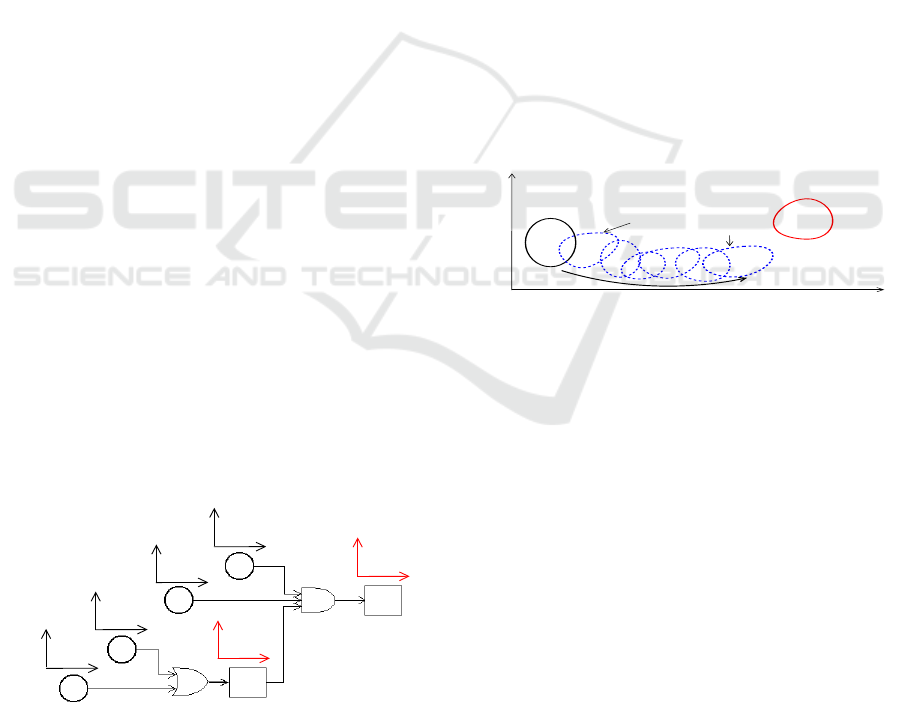
ure 2). The slow drift of an operating mode has for
effect of gradual change of the data from the normal
class to the default class. The goal is to characterize in
term of PFE the drift of an operating mode from the
normal mode to the default mode. For that, we use
AUDyC technique as modelling technique and esti-
mation techniquesof the distances between classes, as
Euclidean and Kullback-Leibler distances. The AU-
DyC technique and the estimation methods of the dis-
tances are presented in the next section.
tances are presented in the next section.
normal mode
de f ault mode
M
j
n
Ω
j
n
M
j
p
Ω
j
p
C
j
n
C
j
p
x
1
x
2
C
j
e
(t
1
)
C
j
e
(t
n
)
Figure 2: Slow drift operating.
3 CURRENT CLASS
MODELLING BY AUDYC
TECHNIQUE
The supervision method based on the AUDyC
technique aims at monitoring each component of the
process and at determining their mode. An operating
mode is represented by a Gaussian class C
j
k
which is
characterized by a center M
j
k
and a matrix of covari-
ance Ω
j
k
. These parameters are estimated in real time
according to the observed data contained into the ob-
servation vector which is denoted X
i
= [x
i
1
,x
i
2
,·· · ,x
i
d
]
in the d space dimensions. The AUDyC algorithm
consists in updating the class parameters recursively
on a sliding window of width N
fen
taking into account
the cardinality of the class C
j
k
, i.e. Card(C
j
k
). The
steps of the algorithm, detailed in (Lecoeuche et al.,
DYNAMICAL CLUSTERING TECHNIQUE TO ESTIMATE THE PROBABILITY OF THE FAILURE OCCURRENCE
OF PROCESS SUBJECTED TO SLOW DEGRADATION
361

2004), are presented thereafter:
• If Card(C
j
k
)=nb ¡ N
fen
: Add information
M
j
k
(t) = M
j
k
(t − 1) +
1
nb+ 1
(X(t) − M
j
k
(t − 1))
Ω
j
k
(t) =
nb− 1
nb
Ω
j
k
(t − 1)+
1
nb+ 1
(X(t) − M
j
k
(t − 1))
⊤
(X(t) − M
j
k
(t − 1))
(2)
• If nb ≥ N
fen
: Add and remove information
M
j
k
(t) = M
j
k
(t − 1) +
1
N
fen
(δX
+
− δX
−
)
Ω
j
k
(t) = Ω
j
k
(t − 1)+
∆X
1
N
fen
1
N
fen
(N
fen
−1)
1
N
fen
(N
fen
−1)
−
(N
fen
+1)
N
fen
(N
fen
−1)
∆X
⊤
(3)
where:
δX
+
= X
new
− M
j
k
(t − 1),
δX
−
= X
old
− M
j
k
(t − 1),
∆X = [δX
+
δX
−
].
(4)
with M
j
k
(t) and Ω
j
k
(t) respectively center and covari-
ance matrix of the class C
j
k
at time t, N
fen
the width
of the sliding window, X
new
= X(t), X
old
the old data
in the set affected to C
j
k
.
Then, the distances between the normal, current
and default classes can be computed according to the
center and the covariance matrix of each class. The
Euclidean distance corresponds to the distance be-
tween the center of two classes:
d
Eu
= (M
j
1
− M
j
2
)
⊤
(M
j
1
− M
j
2
)
(5)
where M
j
1
and M
j
2
are the centers of the classes C
j
1
and
C
j
2
respectively.
The Kullback-Leibler distance corresponds to the dis-
tance between two classes taking into account their
shape, i.e. the covariance matrices, (Kullback and
Leibler, 1951). In the general case (Anguita and Her-
nando, 2004), the distance between the classes C
j
1
and
C
j
2
is expressed by:
d
kl
(C
j
1
,C
j
2
) =
1
2
(M
j
1
−M
j
2
)
⊤
(Ω
−1
1
+Ω
−1
2
)(M
j
1
−M
j
2
)
+
1
2
trace(Ω
−1
1
Ω
2
+ Ω
1
Ω
−1
2
) − d. (6)
where d is the dimension of the data representation
space, Ω
1
= Ω
j
1
and Ω
2
= Ω
j
1
are the covariance ma-
trices of the classes C
j
1
and C
j
2
. The second term of
d
kl
, i.e. trace( ), is specifically impacted by the shape
and the orientation of the classes.
Finally, the distances between the several modes are
used to estimate the probabilities of the failure occur-
rence of each component, as detailed in the next sec-
tion.
4 ESTIMATION OF FAILURE
OCCURRENCE
PROBABILITIES
The probability of the failure occurrence, denoted
p
E
j
(t), is defined as the PFE of an elementary com-
ponent, and is considered as an indicator of the dete-
rioration of this component. It is estimated according
to the distance covered by the current class towards
the default class, α(t), due to slow drifts:
p
E
j
(t) = 1 − α(t) (7)
with:
α(t) =
distance(C
j
p
,C
j
e
(t))
distance(C
j
n
,C
j
p
)
(8)
where C
j
n
, C
j
p
, and C
j
e
are the normal, default and
current classes. The distance between two classes
is computed according to the Euclidean (5) or the
Kullback-Leibler (6) methods. It is assumed that
0 ≤ α(t) ≤ 1.
• Estimation of p
E
j
(t) based on Euclidean Dis-
tance
The percentage of distance α
Eu
(t) which is estimated
according to the Euclidean distance (5), is used to de-
termine the probability p
E
j
Eu
(t) according to the rela-
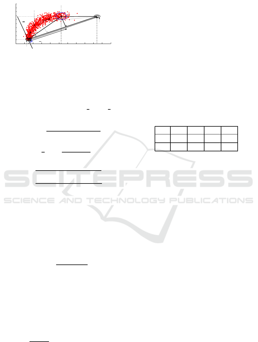
tion (7). The example shown in Figure 3 is considered
to illustrate this method. Three classes for component
j are represented: normal C
j
n
, current C
j
e
, and default
C
j
p
classes characterized by (M
j
n
, Ω
j
n
), (M
j
e
, Ω
j
e
), and
(M
j
p
, Ω
j
p
), respectively.
The percentage of distance α
Eu
(t) at each time t is
given by:
α
Eu
(t) =
d
Eu
(M
j
p
,M
′ j
e
(t))
d
Eu
(M
j
n
,M
j
p
)
(9)
where the distances d
Eu
are expressed by relation (5),
and M
′ j
e
is the orthogonal projection of the center M
j
e
on the segment [M
j
n
M
j
p
]. The distance d
Eu
(M
j
n
,M
j
p
) =
ICINCO 2009 - 6th International Conference on Informatics in Control, Automation and Robotics
362
4 5 6 7 8 9 10 11 12 13 14 15
4
5
6
7
8
9
10
11
12
13
14
+
+
D
j
M
j
p
M
j
n
M
j
e
Ω
j
n
Ω
j
p
Ω
j
e
normal mode
de f ault mode
Dri f t operation
Center o f the evolutive f unctioning mode (C
j
e
)
x
1
x
2
β
π
2
−
π
2
x
j
y
j
z
j
Figure 3: Evolution of a class from the normal class to the
Figure 3: Evolution of a class from the normal class to the
default class.
D
j
is constant (10). The distance d
Eu
(M
j
n
,M
′ j
e
(t)) =
x
j
is determined according to relation (11) from the
triangle formed by the centers of the classes (see Fig-
ure 3). It is assumed that the current class can only
evolve towards the default class. Consequently, the
angle β is always include between −
π
2
< β <
π
2
, and
the orthogonal projection of the center M
j
e
is always
included in the segment [M
j
n
M
j
p
].
D
j
=
q
(M
j
n
− M
j
p
)
⊤
(M
j
n
− M
j
p
) (10)
x
j
(t) =
1
2
"
D
j
+
y
2
j
(t) − z
2
j
(t)
D
j
#
(11)
with:
y
j
(t) =
q
(M
j
n
− M
j
e
(t))
⊤
(M
j
n
− M
j
e
(t)) (12)
z
j
(t) =
q
(M
j
p
− M
j
e
(t))
⊤
(M
j
p
− M
j
e
(t)) (13)
(14)
• Estimation of p
E
j
(t) based on Kullback-Leibler
Distance
The Kullback-Leibler distance is used to estimate the
percentage of distance α
Kl
(t) and then to determine
the probability p
E
j
Kl
(t), according to the relation (7).
The percentage of distance α
Kl
(t) at each time t is
given by:
α
kl
(t) =
d
kl
(C
j
p
,C
j
e
(t))
d
kl
(C
j
n
,C
j
p
)
(15)
where the distances d
kl
are expressed by relation (6).
The Kullback-Leibler distance between the class C
j
n
and the class C
j
p
is constant.
The percentage of distance α
Kl
(t) is computed
only when the current class C
j
e
evolves towards the
default class C
j
p
. A criterion T
d
c
is defined to verify
this condition (16). Thus, α
Kl
(t) is computed if and
only if the criterion T
d
c
is strictly negative.
T
d
c
=
1
N
fen
− 1
N
fen
∑
t=2
sign(∆t),
∆(t) = d
kl
(C
j
p
,C
j
e
(t)) − d
kl
(C
j
p
,C
j
e
(t − 1))
(16)
• Interpretation of p
E
j
(t) Computed According
to Euclidean and Kullback-Liebler Distances
The probabilities p
E
j
Eu
(t) and p
E
j
Kl
(t) are computed
according to the Euclidean or Kullback-Liebler dis-
tances α
Eu
(t) and α
Kl
(t). To interprete and verify
the pertinence of these indicators and thus the pro-
posed methods, a scenario which consists in four cur-
rent classes C
j
1
to C
j
4
which evolve to the normal class
C
j
n
towards the default class C
j
p
, is considered and de-
picted in Figure 4. The classes C
j
1
, C
j
2
and C
j
3
have the
same centers but their matrices of covariance are dif-
ferent. The class C
j
4
is characterized by different cen-
ter and covariance matrice. The probabilities p
E
j
Eu
(t)
and p
E
j
Kl
(t) are computed for the four classes. The re-
sults are given in Table 1.
Table 1: Probabilities computed for the classes.
C
j
1
C
j
2
C
j
3
C
j
4
p
E
j
Eu
0,50 0,50 0,50 0,56
p
E
j
Kl
0,36 0,50 0,46 0,46
The Euclidean distance leads to the estimation of a
same pourcentage p
E
j
Eu
for classes C
j
1
, C
j
2
and C
j
3
, and
to a pourcentage more important for the class C
j
4
. In-
deed, the center of the classC
j
4
is nearest to the default
class than the others classes C
j
p
. This distance is eas-
ily interpretable but it does not take into account the
shape and the orientation of the classes.
The Kullback-Lieblerdistance leads to the estima-
tion of pourcentages p
E
j
Kl
different for the classes C
j
1
,
C
j
2
and C
j
3
. Although, the covariance matrix of the
class C
j
1
is smaller than the covariance matrix of the
class C
j
3
, the difference between the obtained pour-
centages seems to be too important, and these indica-
tors are not directly interpretable as the probabilities
of the failure occurrence. Moreover, the pourcentages
p
E
j
Kl
of the classes C
j
3
and C
j
4
are identical although
the class C
j
4
is nearest of the default class (see Figure
4). Finally, the Kullback-Liebler distance allows to
take into account the shape and the orientation of the
classes, but it is not directly usable for the estimation
of the probabilities of the failure occurrence.
• New Estimation Method of p
E
j
(t)
A new estimation method of the probability p
E
j
(t) is
proposed to provide pertinent indicators which take
into account in priority the position of the classes,
but also, the remoteness, enlarging and rotation of
these classes. It consists in a weigthed combination of
p
E
j
Eu
(t) computed according to Euclidean distance and
DYNAMICAL CLUSTERING TECHNIQUE TO ESTIMATE THE PROBABILITY OF THE FAILURE OCCURRENCE
OF PROCESS SUBJECTED TO SLOW DEGRADATION
363
5 10 15 20 25 30 35 40 45 50 55 60
0
5
10
15
20
C
j
n
C
j
1
C
j
3
C
j
2
C
j
4
C
j
p
Figure 4: Scenario of evolution of classes from a normal
class towards a default class.
p
ε
which is computed according to the second term
of the Kullback-Leibler distance (6). The probability
p
E
j
(t) is expressed as:
p
E
j
(t) = p
E
j
Eu
(t) + λ p
ε
(17)
where λ (0 < λ < 1) is a weight coefficient. The pa-
rameter p
ε
is function of the covariances matrices of
the normal, default and current classes:
p
ε
=
T
1
T
1
+ T
2
T
1
= trace(Ω
e
Ω
−1
p
+ Ω
−1
e
Ω
p
)
T
2
= trace(Ω
p
Ω
−1
n
+ Ω
−1
p
Ω
n
)
(18)
The coefficient λ is tuned in order to take into
account the covariance matrices in the estimation
of p
E
j
(t) without however obtaining too important
differences between the distances from the classes.
In Table 2, we presente the occurrence probabilities
computed by relation (17) according to λ = 1/10.
Table 2: Failure occurrence probabilities.
C
j
1
C
j
2
C
j
3
C
j
4
p
E
j
(t)
0,53 0,55 0,54 0,60
If the value of λ is too small, the shape of the class
is not taken into account, and that leads at consid-
ering only the Euclidean distance. If the value of λ
is too big, the shape of the class has too much influ-
ence on the estimation of p
E
j
(t), and that leads to the
same problem of interpretation than the distance of
Kullback-Leibler. The proposed method is applied on
a real scenario in the next section.
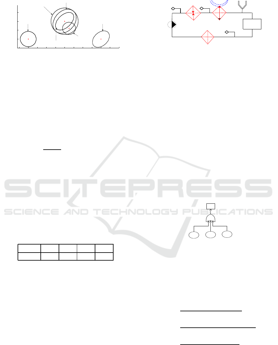
5 APPLICATION
A temperature controller is a process which is used to
control the temperature of a client system. It is com-
posed of an electric heater, a pump, a heat exchanger
and a filter (see Figure 5). The components of this
heater
exchanger
Filter
Pump
client
system
expansion
tank
sensor
coldwater
Figure 5: Thermo-regulator components.
process are subject to failures related to slow degra-
dations due to scaling and fouling essentially. If these
failures are not taken into account early enough, they
can cause the stop of the process.
The first step is the FMEA of the temperature con-
troller which allows the determination of the Fault
Tree of the process (see Figure 6). The Fault Tree
is composed of three basic events associated to each
component and a top event which correspond to the
no temperature control. The basic events are:
• Failure of the heater (E
1
)
• Failure of the exchanger (E
2
)
• Failure of the filter (E
3
)
the top event is:
• No temperature control (E
4
)
E
1
E
2
E
3
E
4
Figure 6: Fault Tree of the temperature controller.
The temperature controller is equipped by sensors
located at the input and output of each component.
These sensors measure the pressure of the fluid. An
observation vector is done by X
1
= (x
1
,x
2
,x
3
)
⊤
where
the three indicators are determined according to the
measurements:
x
1
=
P
input heater
− P
output heater
∆P
pump
(19)
x
2
=
P
input exchanger
− P
output exchanger
∆P
pump
(20)
x
3
=
P
input filter
− P
output pump
∆P
pump
(21)
where x
1
, x
2
, x
3
are indicators to monitor the heater,
the exchanger and the filter respectivelly.
The AUDyC technique allows the monitoring of
elementary components of the temperature controller.
ICINCO 2009 - 6th International Conference on Informatics in Control, Automation and Robotics
364

The estimation method of the occurrence probabili-
ties, with a weight coefficient tuned as λ = 1/20, λ =
1/50, is used to estimate in real time the p
E
j
(t)
j= 1,2,3
(17) of each elementary component, and finally the
PFE of top event (E
4
) by propagation the basic
events.
where the events E
1
, E
2
and E
3
are independents.
Thus, the PFE of the event E
4
is expressed as:
PFE(E
4
) = ((p
E
4
(t
1
),t
1
),··· ,(p
E
4
(t
n
),t
n
)) (22)
In the real scenario considered, the components of the
temperature controller are subjected to drifts as de-
picted in Figure 7. The PFE(E
4
) determined accord-
ing to the relation (22) are displayed in Figure 8. On
this real scenario,the tune λ = 1/20 leads to a too im-
portant influence of p
ε
, whereas λ = 1/50 presents a
good compromise. La figure 8.a montre l’influence de
la forme de la classe alors que la figure 8.b l’influence
de la forme de la classe est moins important.
−10
−5
0
5
10
15
20
−10
−5
0
5
10
15
20
25
30
−30
−20
−10
0
10
x
1
x
2
x
3
Heater failure
exchanger failure
Filter failure
Normal class
Figure 7: Drifts of operating of the components.
0 100 200 300 400 500 600 700 800
0
0.1
0.2
0.3
0.4
0.5
0.6
0.7
0.8
0 100 200 300 400 500 600 700 800
0
0.1
0.2
0.3
0.4
0.5
0.6
0.7
0.8
PFE(E
4
)
PFE(E
4
)
PFE
Eu
PFE
Eu
PFE
PFE
(a)
(b)
Time
PFE E
Figure 8: PFE(E
4
) according to (a) λ = 1/20, (b) λ = 1/50.
6 CONCLUSIONS
The supervision method proposed in this paper al-
lows the estimation of the probability of failure occur-
rence of processes in real time. The dynamic cluster-
ing method is used to track the evolution of operating
modes of processes by determining the characteristics
of each class (center and covariance matrix).
The center and the covariance matrix being
adapted by AUDyC, the Euclidean distance and trace
of the covariance matrices are used to estimate the
probability of the failure occurrence. The Euclidean
distance does not allow to take into account the shape
and the orientation of the class, and the Kullback-
Leibler distance, are not easily interpretable. Then,
a new method which is based on the weight combi-
nation between the probabilities estimated with the
Euclidean distance and with the trace of the covari-
ance matrices, is proposed and illustrated on real case.
In futur works, we will propose a prognosis strategy
based on this method to forecast the occurrence prob-
ability of events, and a step to tune the weight coef-
ficients of the proposed method. The goal is to de-
termine indicators to improve the predictive mainte-
nance of processes. This will be implemented for pre-
dictive maintenance of the temperature controller and
of measure the apport of the proposed methods.
REFERENCES
Anguita, J. and Hernando, J. (2004). Inter-phone and inter-
word distances for confusability prediction in speech
recognition. Congreso de la Sociedad Espaola para
el Procesamiento del Lenguaje Natural, (33):33–40.
Desinde, M., Flaus, J. M., and Ploix, S. (2006). Tool and
methodology for online risk assessement of process.
In Lambda-Mu 15 /Lille.
Grall, A., Berenguer, C., and Dieulle, L. (2002). A
condition-based maintenance policy for stochastically
deteriorating systems. Reliability Engineering and
System Safety, 76(2):167–180.
Kullback, S. and Leibler, R. A. (1951). On information and
sufficiency. Annal of Mathematical Statistics,22:79-
86.
Lassagne, M. (2000). Applying a decision-analysis-based
method to the evaluation of potential risk-reducing
measures : The case of a floating production storage
and offloading unit in the gulf of mexico. SPE annual
technical conference, Dallas TX , USA.
Lecoeuche, S., Lurette, C., and Lalot, S. (2004). New su-
pervision architecture based on on-line modelling of
non-stationary data. Neural Computing and Applica-
tions Journal, 13:323–338.
Lurette, C. and Lecoeuche, S. (2003). Unsupervised and
auto-adaptive neural architecture for on-line monitor-
ing. application to a hydraulic process. Engineering
Applications of Artificial Intelligence, 16:441–451.
Mouchawed, S. M. and Billaudel, P. (2002). Influence of
the choice of histogram parameters at fuzzy pattern
matching performance, int. journal of wseas transac-
tions on system. WSEAS Transactions on Systems,
1:260–266.
Muller, A., Suhner, M.-C., Iung, B., and Morel, G. (2004).
Prognosis-based maintenance decision-making for
industrial process performance optimisation. In
7th IFAC Symposium on Cost Oriented Automation
(COA2004). Gatineau/Ottawa Canada.
Vesely, W. E., Goldberg, F. F., Robert, N. H., and Haasl,
D. F. (1981). Fault Tree Handbook. US nuclear Reg-
ulatory Commission, Washington D.C., USA.
DYNAMICAL CLUSTERING TECHNIQUE TO ESTIMATE THE PROBABILITY OF THE FAILURE OCCURRENCE
OF PROCESS SUBJECTED TO SLOW DEGRADATION
365
