
SUMMARIZING SETS OF CATEGORICAL SEQUENCES
Selecting and Visualizing Representative Sequences
Alexis Gabadinho, Gilbert Ritschard, Matthias Studer and Nicolas S. Müller
Department of Econometrics and Laboratory of Demography, University of Geneva
40, bd du Pont-d’Arve, CH-1211 Geneva, Switzerland
Keywords:
Categorical sequence data, Representativeness, Dissimilarity, Discrepancy of sequences, Summarizing sets of
sequences, Visualization.
Abstract:
This paper is concerned with the summarization of a set of categorical sequence data. More specifically, the
problem studied is the determination of the smallest possible number of representative sequences that ensure a
given coverage of the whole set, i.e. that have together a given percentage of sequences in their neighborhood.
The goal is to yield a representative set that exhibits the key features of the whole sequence data set and
permits easy sounded interpretation. We propose an heuristic for determining the representative set that first
builds a list of candidates using a representativeness score and then eliminates redundancy. We propose also a
visualization tool for rendering the results and quality measures for evaluating them. The proposed tools have
been implemented in TraMineR our R package for mining and visualizing sequence data and we demonstrate
their efficiency on a real world example from social sciences. The methods are nonetheless by no way limited
to social science data and should prove useful in many other domains.
1 INTRODUCTION
Sequences of categorical data appear in many dif-
ferent scientific fields. In the social sciences,
such sequences are mainly ordered list of states
(employed/unemployed) or events (leaving parental
home, marriage, having a child) describing individ-
ual life trajectories, typically longitudinal biographi-
cal data such as employment histories or family life
courses.
One widely used approach for extracting knowl-
edge from such sets consists in computing pair-
wise distances by means of sequence alignment al-
gorithms, and next clustering the sequences by using
these distances. This method has been applied to var-
ious data since the pioneering work of (Abbott and
Forrest, 1986). A review can be found in (Abbott and
Tsay, 2000). The expected outcome of such a strat-
egy is a typology, with each cluster grouping cases
with similar patterns (trajectories).
An important aspect of sequence analysis is also
to compare the patterns of cases grouped according to
the values of covariates (for instance sex or socioeco-
nomic position in the social sciences).
A crucial task is then to summarize groups of se-
quences by describing the patterns that characterize
them. This could be done by resorting to graphi-
cal representations such as sequence index plots, state
distribution plots or sequence frequency plots (Müller
et al., 2008). However, relying on these graphical
tools suffers from some drawbacks. Sequence in-
dex plots give a (sorted) view of all the sequences in
each subset and assigning them a meaning is mainly
a subjective task. State distribution plots are ag-
gregated transversal views that occult individual se-
quences and their interpretation can be misleading.
Sequence frequency plots that focus on the most fre-
quent sequences provide only a partial view especially
when there is a great number of distinct sequences.
Hence, we need more appropriate tools for ex-
tracting the key features of a given subset or data par-
tition. We propose an approach derived from the con-
cept of representative set used in the biological sci-
ences (Hobohm et al., 1992; Holm and Sander, 1998).
The aim in this field is mainly to get a reduced refer-
ence base of protein or DNA sequences for optimizing
the retrieval of a recorded sequence that resembles to
a provided one. In this setting, the representative set
must have “maximum coverage with minimum redun-
dancy” i.e. it must cover all the spectrum of distinct
sequences present in the data, including “outliers”.
Our goal is similar regarding the elimination of re-
62
Gabadinho A., Ritschard G., Studer M. and Müller N. (2009).
SUMMARIZING SETS OF CATEGORICAL SEQUENCES - Selecting and Visualizing Representative Sequences.
In Proceedings of the International Conference on Knowledge Discovery and Information Retrieval, pages 62-69
DOI: 10.5220/0002300400620069
Copyright
c
SciTePress

Table 1: List of states in the mvad data set.
1 EM Employment
2 FE Further education
3 HE Higher education
4 JL Joblessness
5 SC School
6 TR Training
dundancy. It differs, however, in that we consider in
this paper representative sets with a user controlled
coverage level, i.e. we do not require maximal cover-
age. We thus define a representative set as a set of non
redundant“typical” sequences that largely, though not
necessarily exhaustively covers the spectrum of ob-
served sequences. In other words, we are interested
in finding a few sequences that together summarize
the main traits of a whole set.
We could imagine synthetic — not observed —
typical sequences, in the same way as the mean of a
series of numbers that is generally not an observable
individual value. However, the sequences we deal
with in the social sciences (as well as in other fields)
are complex patterns and modeling them is difficult
since the successive states in a sequence are most of-
ten not independent of each other. Defining some
virtual non observable sequence is therefore hardly
workable, and we shall here consider only representa-
tive sets constituted of existing sequences taken from
the data set itself.
Since this summarizing step represents an impor-
tant data reduction, we also need indicators for as-
sessing the quality of the selected representative se-
quences. An important aspect is also to visualize
these in an efficient way.
Such tools and their application to social science
data are presented in this paper. These tools are new
features of our TraMineR library for mining and visu-
alizing sequences in R (Gabadinho et al., 2009).
2 DATA
To illustrate our purpose we consider a data set
from (McVicar and Anyadike-Danes, 2002) stem-
ming from a survey on transition from school to work
in Northern Ireland. The data contains 70 monthly
activity state variables from July 1993 to June 1999
for 712 individuals. The alphabet is made of 6 states
detailed in Table 1.
The three first sequences of this data set repre-
sented as distinct states and their associated durations
(the so called State Permanence Format) look as fol-
lows
Sequence
[1] EM/4-TR/2-EM/64
[2] FE/36-HE/34
[3] TR/24-FE/34-EM/10-JL/2
We consider in this paper the outcome of a cluster
analysis of the sequences based on Optimal Match-
ing (OM). The OM distance between two sequences x
and y, also known as edit or Levenshtein distance, is
the minimal cost in terms of indels — insertions and
deletions — and substitutions necessary to transform
x into y. We computed the distances using a substitu-
tion cost matrix based on transition rates observed in
the data set and an indel cost of 1. The clustering is
done with an agglomerative hierarchical method us-
ing the Ward criterion. A four cluster solution is cho-
sen. Table 2 indicates some descriptive statistics for
each of the clusters.
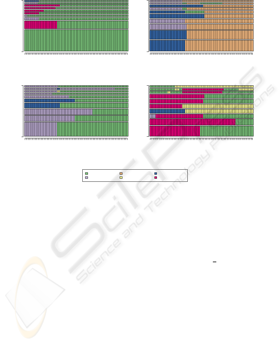
The sequence frequency plots in Fig. 1 displays
the 10 most frequent sequences in each cluster and
give a first idea of their content. The bar widths
are proportional to the sequence frequencies. The 10
most frequent sequences represent about 40% of all
the sequences in cluster 1 and 2, while this proportion
is 27% and 21% for clusters 3 and 4 due to a higher
diversity of the patterns.
3 METHODS
Our aim is to find a small subset of non redundant se-
quences that ensures a given coverage level, this level
being for instance defined as the percentage of cases
that are within a given neighborhood of at least one of
the representative sequences. We propose an heuristic
for determining such a representative subset.
It works in two main steps. In the first stage it
prepares a sorted list of candidate representative se-
quences without caring for redundancyand eliminates
redundancy within this list in a second stage. It basi-
cally requires the user to specify a representativeness
criterion for the first stage and a similarity measure
for evaluating redundancy in the second one.
Table 2: Number of cases, distinct sequences and discrep-
ancy within each cluster.
N Dist. seq. Discr.
Cluster 1 265 165 18.3
Cluster 2 153 88 23.5
Cluster 3 194 148 27.9
Cluster 4 100 89 37.2
SUMMARIZING SETS OF CATEGORICAL SEQUENCES - Selecting and Visualizing Representative Sequences
63
Cluster 1
Cum. % freq. (n=265)
Sep.93 Jul.94 Apr.95 Jan.96 Oct.96 Jul.97 Apr.98 Jan.99
0% 37.7%
Cluster 2
Cum. % freq. (n=153)
Sep.93 Jul.94 Apr.95 Jan.96 Oct.96 Jul.97 Apr.98 Jan.99
0% 41.2%
Cluster 3
Cum. % freq. (n=194)
Sep.93 Jul.94 Apr.95 Jan.96 Oct.96 Jul.97 Apr.98 Jan.99
0% 26.8%
Cluster 4
Cum. % freq. (n=100)
Sep.93 Jul.94 Apr.95 Jan.96 Oct.96 Jul.97 Apr.98 Jan.99
0% 21%
employment
further education
higher education
joblessness
school
training
Figure 1: 10 most frequent sequences within each cluster.
3.1 Sorting Candidates
The initial candidate list is made of all distinct se-
quences appearing in the data. Since the second stage
will extract non redundant representative sequences
sequentially starting with the first element in the list,
sorting the candidates according to a chosen represen-
tativeness criterion ensures that the “best” sequences
given the criterion will be included. We present here
five alternatives for measuring the sequence represen-
tativeness.
Sequence Frequency. A first simple criterion is to
sort the sequences according to their frequency. The
more frequent a sequence the more representative it
is supposed to be. Hence, sequences are sorted in de-
creasing frequency order.
Neighborhood Density. A second criterion is
the number — the density — of sequences in the
neighborhood of each candidate sequence. This
requires indeed to set the neighborhood diameter.
We suggest to set it as a given proportion of the
maximal theoretical distance between two sequences.
Sequences are sorted in decreasing density order.
Mean State Frequency. A third criterion is the mean
value of the transversal frequencies of the successive
states. Let s = s
1
s
2
···s
ℓ
be a sequence of length ℓ and
( f
s
1
, f
s
2
,..., f
s
ℓ
) the frequencies of the states at time
(t
1
,t
2
,...t
ℓ
). The mean state frequency is the sum of
the state frequencies divided by the sequence length
MSF(s) =
1
ℓ
ℓ
∑
i=1
f
s
i
The lower and upper boundaries of MSF are 0 and 1.
MSF is equal to 1 when all the sequences in the set are
the same, i.e. when there is a single distinct sequence.
The most representative sequence is the one with the
highest score.
Centrality. A classical representative of a data set
used in cluster analysis is the medoid. It is defined
as the most central object, i.e. the one with minimal
sum of distances to all other objects in the set (Kauf-
man and Rousseeuw, 1990). This suggests to use the
sum of distances to all other sequences, i.e. the cen-
trality as a representativeness criterion. The smallest
the sum, the most representative the sequence. It may
be mentioned that the most central observed sequence
KDIR 2009 - International Conference on Knowledge Discovery and Information Retrieval
64

is also the nearest from the ‘virtual’ true center of the
set (Studer et al., 2009).
Sequence likelihood. The sequence likelihood P(s)
is defined as the product of the probability with which
each of its observed successive state is supposed to
occur at its position. Let s = s
1
s
2
···s
ℓ
be a sequence
of length ℓ. Then
P(s) = P(s
1
,1) · P(s
2
,2)···P(s
ℓ
,ℓ)
with P(s
t
,t) the probability to observe state s
t
at posi-
tion t. The question is how to determinate the state
probabilities P(s
t
,t). One commonly used method
for computing them is to postulate a Markov model,
which can be of various order. Below, we just con-
sider probabilities derivedfrom the first order Markov
model, that is each P(s
t
,t), t > 1 is set to the transi-
tion rate p(s
t
|s
t−1
) estimated across sequences from
the observations at positions t and t −1. For t = 1, we
set P(s
1
,1) to the observed frequency of the state s
1
at
position 1. The likelihood P(s) being generally very
small, we use −logP(s) as sorting criterion. The lat-
ter quantity is minimal when P(s) is equal to 1, which
leads to sort the sequences in ascending order of their
score.
3.2 Eliminating Redundancy
Once a sorted list of candidates has been defined, the
second stage consists in eliminating redundancy since
we do not want our representative set to contain simi-
lar sequences. The procedure is as follows:
• Select the first sequence in the candidate list (the
best one given the chosen criterion);
• Process each next sequence in the sorted list of
candidates. If this sequence is similar to none of
those already in the representative set, that is dis-
tant from more than a predefined threshold from
all of them, add it to the representative set.
The threshold for sequence similarity is defined as
a proportion of the maximal theoretical distance. For
the OM distance this theoretical maximum is for two
sequences (s
1
,s
2
) of length (ℓ
1
,ℓ
2
)
D
max
= min(ℓ
1
,ℓ
2
) · min
2C
I
,max(S)
+ |ℓ
1
− ℓ
2
| ·C
I
where C
I
is the indel cost and maxS the maximal sub-
stitution cost.
3.3 Size of the Representative Set
Limiting our representative set to the mere se-
quence(s) with the best representative score may lead
to leave a great number of sequences badly repre-
sented. Alternatively, proceeding the complete list of
candidates to achieve a full coverage of the data set is
not a suitable solution since we look for a small set of
representative sequences.
To control the size of the representative set, we
limit the size of the candidate list so that the cu-
mulated frequency of the retained distinct candidates
reaches a threshold proportion trep of the whole data
set. Setting for instance trep = 25% ensures that at
least 25% of the sequences will have a representative
in their neighborhood and that the final representative
set will contain at most 25% of the distinct sequences
in the whole set. Thus trep defines also a minimum
coverage level.
There are indeed other possible ways of control-
ling the size of the representative set such as fixing a)
the number or the proportion of sequences in the final
representative set, or b) the desired coverage level.
3.4 Measuring Quality
A first step to define quality measures for the repre-
sentative set is to assign each sequence to its nearest
representative according to the considered pairwise
distances. Let r
1
...r
nr
be the nr sequences in the repre-
sentative set and d(s,r
i
) the distance between the se-
quence s and the ith representative. Each sequence s is
assigned to its closer representative. When a sequence
is equally distant from two or more representatives,
the one with the highest representativeness score is
selected. Hence, letting n be the total number of se-
quences and na
i
the number of sequences assigned to
the ith representative, we have n =
∑
nr
i=1
na
i
. Once
each sequence in the set is assigned to a representa-
tive, we can derive the following quantities from the
pairwise distance matrix.
Mean distance. Let SD
i
=
∑
na
i
j=1
d(s
j
,r
i
) be the sum
of distances between the ith representative and its na
i
assigned sequences. A quality measure is then
MD
i
=
SD
i
na
i
the mean distance to the ith representative.
Coverage. Another quality indicator is the number of
sequences assigned to the ith representative that are in
its neighborhood, that is within a distance dn
max
nb
i
=
na
i
∑
j=1
d(s
j
,r
i
) < dn
max
.
The threshold dn
max
is defined as a proportion of
D
max
. The total coverage of the representative set is
the sum nb =
∑
nr
i
nb
i
expressed as a proportion of the
number n of sequences, that is nb/n.
Distance gain. A third quality measure is obtained
by comparing the sum SD
i
of distances to the ith rep-
SUMMARIZING SETS OF CATEGORICAL SEQUENCES - Selecting and Visualizing Representative Sequences
65
resentative to the sum DC
i
=
∑
na
i
j=1
d(s
j
,c) of the dis-
tances of each of the na
i
sequences to the center of
the complete set. The idea is to measure the gain of
representing those sequences by their representative
rather than by the center of the set. We define thus the
quality measure Q
i
of the representative sequence r
i
as
Q
i
=
DC
i
− SD
i
DC
i
which gives the relative gain in the sum of distances.
Note that Q
i
may be negative in some circumstances,
meaning that the sum of the na
i
distances to the repre-
sentative r
i
is higher than the sum of distances to the
true center of the set. A similar measure can be used
to assess the overall quality of the representative set,
namely
Q =
∑
nr
i
DC
i
−
∑
nr
i
SD
i
∑
nr
i
DC
i
=
nr
∑
i=1
DC
i
∑
j
DC
j
Q
i
.
Discrepancy. A last quality measure is the sum SC
i
=
∑
na
i
j=1
d(s
j
,c
i
) of distances to the true center c
i
of the
na
i
sequences assigned to r
i
, or the mean of those dis-
tances V
i
= SC
i
/na
i
, which can be interpreted as the
discrepancy of the set (Studer et al., 2009).
4 RESULTS
A graphical tool for visualizing the selected represen-
tative sequences together with information measures
is included in the TraMineR package. A single func-
tion produces a “representative sequence plot” (Fig-
ure 2) where the representative sequences are plotted
as horizontal bars with width proportional to the num-
ber of sequences assigned to them. Sequences are
plotted bottom-up according to their representative-
ness score. Above the plot, two parallel series of sym-
bols associated to each representative are displayed
horizontally on a scale ranging from 0 to the max-
imal theoretical distance D
max
. The location of the
symbol associated to the representative r
i
indicates on
axis A the (pseudo) variance (V
i
) within the subset of
sequences assigned to r
i
and on the axis B the mean
distance MD
i
to the representative.
4.1 Key Patterns
The set of representative sequences found with the se-
quence frequencycriterion is displayed in Figure 2 for
each of the four clusters of our example. The plots
give clearly a more readily interpretable view of the
content of the clusters than the frequency plots dis-
played in Figure 1. Detailed statistics about these sets
are presented in Table 3.
Table 3: Representative sequences by cluster, frequency cri-
terion, trep=25%.
na (%) nb (%) MD V Q
Cl. 1
r
1
116 43.8 66 24.9 12.5 9.9 14.5
r
2
101 38.1 34 12.8 17.3 13.3 17.0
r
3
48 18.1 21 7.9 19.2 14.5 11.5
r
1−3
265 100.0 121 45.7 15.6 18.3 15.0
Cl. 2
r
1
62 40.5 35 22.9 11.9 9.0 30.5
r
2
63 41.2 24 15.7 20.4 13.9 30.6
r
3
28 18.3 10 6.5 18.3 12.1 24.5
r
1−3
153 100.0 69 45.1 16.6 23.5 29.4
Cl. 3
r
1
54 27.8 41 21.1 10.3 8.3 41.3
r
2
47 24.2 21 10.8 22.8 17.1 -11.6
r
3
56 28.9 18 9.3 31.0 22.1 8.9
r
4
22 11.3 10 5.2 31.7 20.1 22.9
r
5
15 7.7 4 2.1 28.1 19.0 38.7
r
1−5
194 100.0 94 48.5 23.1 27.9 17.0
Cl. 4
r
1
28 28.0 15 15.0 15.0 10.9 50.4
r
2
12 12.0 4 4.0 17.8 12.7 53.3
r
3
7 7.0 4 4.0 20.6 14.4 63.9
r
4
15 15.0 7 7.0 21.3 15.3 31.7
r
5
2 2.0 2 2.0 6.8 3.4 81.7
r
6
5 5.0 2 2.0 20.7 12.0 48.4
r
7
4 4.0 1 1.0 41.0 24.2 -6.9
r
8
13 13.0 1 1.0 29.4 13.2 39.0
r
9
3 3.0 1 1.0 24.3 15.1 35.3
r
10
6 6.0 1 1.0 41.7 24.3 -19.9
r
11
5 5.0 1 1.0 37.4 20.1 -6.0
r
1−11
100 100.0 39 39.0 22.7 37.2 39.0
The representative sequences were extracted from
a list of candidates sorted in decreasing order of their
frequency. The number of candidates was limited
by setting the trep threshold for the cumulated fre-
quency of the candidates to 25%. The pairwise dis-
tances used are the optimal matching distances that
we used for the clustering. The threshold dn
max
for
similarity (redundancy) between sequences was set as
10% of the maximal theoretical distance D
max
. The
sequence length being ℓ = 70, the indel cost 1 and
the maximal substitution cost 1.9995, we get D
max
=
70· min(2,1.9995) = 139.96.
The first cluster is represented by three sequences.
The first one, employment during the whole period
represents 116 (44%) sequences of the cluster (Ta-
ble 3), and its neighborhood (within 10% of D
max
)
includes 66 (25%) sequences. The second represen-
tative sequence, a spell of training followed by em-
ployment represents 101 (38%) additional cases and
counts 34 (13%) sequences in its neighborhood. The
KDIR 2009 - International Conference on Knowledge Discovery and Information Retrieval
66
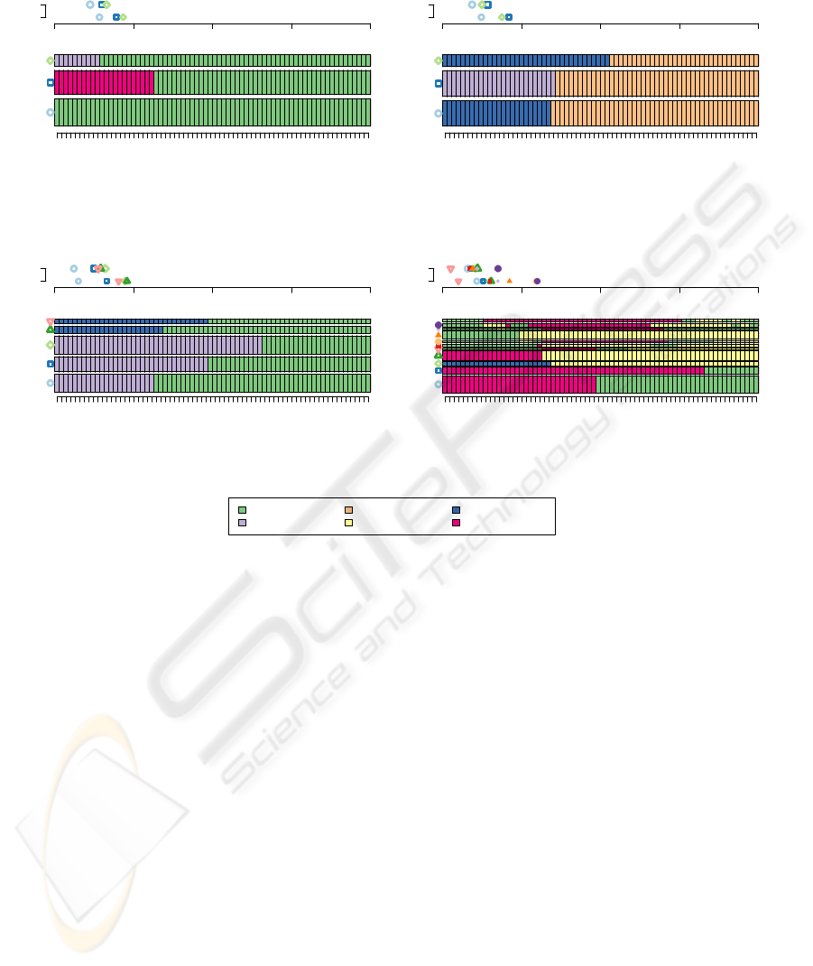
Cluster 1
(N=265)
Sep.93 Jul.94 Apr.95 Feb.96 Dec.96 Oct.97 Jul.98 Apr.99
Criterion=frequency, 121 neighbours (45.7%)
0 22 44 67 89
B
A
(A) Discrepancy (mean dist. to center)
(B) Mean dist. to representative seq.
Cluster 2
(N=153)
Sep.93 Jul.94 Apr.95 Feb.96 Dec.96 Oct.97 Jul.98 Apr.99
Criterion=frequency, 69 neighbours (45.1%)
0 24 49 73 98
B
A
(A) Discrepancy (mean dist. to center)
(B) Mean dist. to representative seq.
Cluster 3
(N=194)
Sep.93 Jul.94 Apr.95 Feb.96 Dec.96 Oct.97 Jul.98 Apr.99
Criterion=frequency, 94 neighbours (48.5%)
0 35 69 104 139
B
A
(A) Discrepancy (mean dist. to center)
(B) Mean dist. to representative seq.
Cluster 4
(N=100)
Sep.93 Jul.94 Apr.95 Feb.96 Dec.96 Oct.97 Jul.98 Apr.99
Criterion=frequency, 39 neighbours (39%)
0 35 70 104 139
B
A
(A) Discrepancy (mean dist. to center)
(B) Mean dist. to representative seq.
employment
further education
higher education
joblessness
school
training
Figure 2: Representative sequences selected with the Frequency criterion, within each cluster (mvad data).
third and last representative sequence exhibits a short
spell of further education followed by employment.
Hence, this cluster is characterized by patterns of
rapid entry into employment. Overall, the distance
to the representative is within 10% of D
max
for 121
(46%) sequences of the cluster. The quality measure
Q (see Section 3.4) is respectively 11.5%, 17% and
14.5% for the three sequences in the set and reaches
15% for the whole set.
The second cluster is described by three patterns
leading to higher education, either starting with a spell
of further education or with school. These three pat-
terns cover together (have in their neighborhood)45%
of the sequences and the overall quality measure for
the representative set is 29%.
The number of selected representative sequences
in cluster 3 and 4 is higher due to a lesser redundancy
in the candidate list. In cluster 3, the pattern is a tran-
sition to employment preceded by long (compared to
Cluster 1) spells of school and/or further education.
In this cluster, the five representative sequences cover
together 48.5% of the sequences, which is the highest
attained value.
The key patterns in cluster 4 was less clear when
looking at the sequence frequency plot (Figure 1).
This group is dominated by long spells of train-
ing leading to employment or joblessness and by
disrupted patterns containing spells of joblessness.
Hence these trajectories can be characterized as less
successful transitions from school to work. The diver-
sity of the patterns is high in this cluster which leads
to the extraction of eleven non redundant sequences
from the candidate list. The selected representative
set covers nonetheless 39% of the cases in the clus-
ter while the quality measure reaches its highest level
(Q = 39%). Indeed the discrepancy is high in this
group (V = 37.2) and representing the sequences with
their assigned representative rather than by the center
of the set significantly decreases the sum of distances.
4.2 Comparing Sorting Criterions
Table 4 summarizes the outcome obtained with each
of the five proposed criteria. The Frequency, Density
SUMMARIZING SETS OF CATEGORICAL SEQUENCES - Selecting and Visualizing Representative Sequences
67
and Likelihood criteria provide results of quite equiv-
alent quality while the Mean State Frequency (MSt-
Freq) and Centrality criteria are clearly less satisfac-
tory.
Table 4: Comparing criterions with trep=25%.
nr nb (%) MD Q
Cluster 1
Frequency 3 121 45.7 15.6 15.0
Density 3 121 45.7 15.6 15.0
Likelihood 3 121 45.7 15.6 15.0
MStFreq 2 82 30.9 25.2 -37.6
Centrality 7 104 39.2 18.1 1.4
Cluster 2
Frequency 3 69 45.1 16.6 29.4
Density 3 69 45.1 16.6 29.4
Likelihood 2 59 38.6 18.7 20.5
MStFreq 4 62 40.5 18.4 21.5
Centrality 3 39 25.5 29.9 -27.2
Cluster 3
Frequency 5 94 48.5 23.1 17.0
Density 6 100 51.5 19.3 30.6
Likelihood 8 105 54.1 18.2 34.8
MStFreq 3 81 41.8 31.2 -12.0
Centrality 4 67 34.5 31.3 -12.4
Cluster 4
Frequency 11 39 39.0 22.7 39.0
Density 11 37 37.0 23.8 35.9
Likelihood 7 42 42.0 26.5 28.8
MStFreq 12 36 36.0 29.3 21.3
Centrality 15 36 36.0 29.8 19.9
Selecting the representative sequences in a candi-
date list sorted according to the distance to the cen-
ter yields poor results in many cases. Indeed select-
ing representatives close from the center of the group
leads to poor representation of sequences that are far
from it. The sometimes bad results yielded with the
Mean State Frequency criterion is attributable to the
nature of this criterion, which focuses on the total of
position-dependant scores while completely ignoring
the sequence structure.
From Table 4, it seems that among the three win-
ners, Density that is always ranked 1st or 2nd is the
best compromise. We may notice, however, that no
criterion yields systematically the smallest number of
representatives.
4.3 Size of the Candidate List
Table 5 presents the results obtained after increasing
the trep threshold for the size of the candidate list to
75%. As a consequence the proportion of well rep-
resented sequences is now at least 75%. This gain
comes however at the cost of a considerable increase
in the number nr of selected representativesequences.
With this high trep, the results obtained with the
Density criterion get the best scores with any of the
three considered quality measures for all four clus-
ters. With Likelihood and Frequency we get results
of a quality close to that yielded by Density, while
the Mean Sate Frequency and Centrality give again
poorer results.
Table 5: Comparing criterions with trep=75%.
nr nb (%) MD Q
Cluster 1
Frequency 58 224 84.5 4.4 76.0
Density 58 230 86.8 3.7 79.6
Likelihood 44 216 81.5 5.2 71.6
MStFreq 39 201 75.8 9.1 50.2
Centrality 40 202 76.2 9.4 48.5
Cluster 2
Frequency 27 129 84.3 5.0 78.9
Density 26 132 86.3 4.6 80.3
Likelihood 18 123 80.4 6.1 74.2
MStFreq 23 122 79.7 7.1 69.6
Centrality 23 119 77.8 8.5 64.0
Cluster 3
Frequency 50 158 81.4 8.2 70.7
Density 58 171 88.1 5.5 80.3
Likelihood 42 157 80.9 8.5 69.6
MStFreq 41 148 76.3 12.3 55.9
Centrality 52 156 80.4 10.4 62.6
Cluster 4
Frequency 48 87 87.0 5.6 84.9
Density 48 87 87.0 5.2 85.9
Likelihood 35 76 76.0 10.1 72.8
MStFreq 41 77 77.0 10.8 71.0
Centrality 46 76 76.0 10.1 72.8
5 CONCLUSIONS
We have presented a flexible method for selecting and
visualizing representatives of a set of sequences. The
method attempts to find the smallest number of rep-
resentatives that achieve a given coverage. Differ-
ent indicators have been considered to measure rep-
resentativeness and the coverage can be evaluated by
means of different sequence dissimilarity measures.
The heuristic can be fine tuned with various thresh-
olds for controlling the trade-off between size and
quality of the resulting representative set. The ex-
periments demonstrated how good our method is for
extracting in an readily interpretable way the main
features from sets of sequences. The proposed tools
KDIR 2009 - International Conference on Knowledge Discovery and Information Retrieval
68

are made available as functions of the TraMineR R-
package and are awaiting to be tested with other data
sets.
ACKNOWLEDGEMENTS
This work is part of the Swiss National Science Foun-
dation research project FN-1000015-122230 “Mining
event histories: Towards new insights on personal
Swiss life courses”.
REFERENCES
Abbott, A. and Forrest, J. (1986). Optimal matching meth-
ods for historical sequences. Journal of Interdisci-
plinary History, 16:471–494.
Abbott, A. and Tsay, A. (2000). Sequence analysis
and optimal matching methods in sociology, Review
and prospect. Sociological Methods and Research,
29(1):3–33. (With discussion, pp 34-76).
Gabadinho, A., Müller, N. S., Ritschard, G., and Studer, M.
(2009). Mining sequence data in R with TraMineR: A
user’s guide. Department of Econometrics and Labo-
ratory of Demography, University of Geneva, Geneva.
Hobohm, U., Scharf, M., Schneider, R., and Sander, C.
(1992). Selection of representative protein data sets.
Protein Sci, 1(3):409–417.
Holm, L. and Sander, C. (1998). Removing near-neighbour
redundancy from large protein sequence collections.
Bioinformatics, 14(5):423–429.
Kaufman, L. and Rousseeuw, P. J. (1990). Finding groups in
data: an introduction to cluster analysis. John Wiley
and Sons, New York.
McVicar, D. and Anyadike-Danes, M. (2002). Predicting
successful and unsuccessful transitions from school
to work by using sequence methods. Journal of the
Royal Statistical Society. Series A (Statistics in Soci-
ety), 165(2):317–334.
Müller, N. S., Gabadinho, A., Ritschard, G., and Studer,
M. (2008). Extracting knowledge from life courses:
Clustering and visualization. In DAWAK 2008, volume
LNCS 5182 of Lectures Notes in Computer Science,
pages 176–185, Berlin Heidelberg. Springer.
Studer, M., Ritschard, G., Gabadinho, A., and Müller,
N. S. (2009). Analyse de dissimilarités par arbre
d’induction. Revue des nouvelles technologies de
l’information RNTI, E-15:7–18.
SUMMARIZING SETS OF CATEGORICAL SEQUENCES - Selecting and Visualizing Representative Sequences
69
