DIFFERENCE OF GAUSSIANS TYPE NEURAL IMAGE FILTERING
WITH SPIKING NEURONS
Sylvain Chevallier and Sonia Dahdouh
LIMSI UPR 3251, University Paris-Sud 11, Orsay, France
Keywords:
Spiking neurons, Image filtering, Edges preservation and enhancement.
Abstract:
This contribution describes a bio-inspired image filtering method using spiking neurons. Bio-inspired ap-
proaches aim at identifying key properties of biological systems or models and proposing efficient implemen-
tations of these properties. The neural image filtering method takes advantage of the temporal integration
behavior of spiking neurons. Two experimental validations are conducted to demonstrate the interests of this
neural-based method. The first set of experiments compares the noise resistance of a convolutional difference
of Gaussians (DOG) filtering method and the neuronal DOG method on a synthetic image. The other exper-
iment explores the edges recovery ability on a natural image. The results show that the neural-based DOG
filtering method is more resistant to noise and provides a better edge preservation than classical DOG filtering
method.
1 INTRODUCTION
The term bio-inspired usually refers to the process of
identifyingkey mechanisms of biological systems and
proposing their efficient implementation in an artifi-
cial system.
In vision, it has been identified that an essential
mechanism of the biological visual system is visual
attention. This mechanism allows biological organ-
isms to select only small regions of their visual envi-
ronment and to iteratively process these regions.
The interest of this type of phenomenon for com-
puter vision is obvious. From a computational point
of view, visual attention is a process which allows
to reduce the complexity required to process a visual
scene (Tsotsos, 1989; Tsotsos, 1990; Itti et al., 2005)
which leads to better and sometimes faster results than
classical imaging algorithms.
Artificial attention-based systems could be found
in various applications, such as driver assistance sys-
tems (Michalke et al., 2008), medical image comput-
ing (Fouquier et al., 2008) or robotics (Frintrop et al.,
2006). All those type of applications are based on the
identification of salient regions. Those type of regions
are the ones selected by the attention-based systems
as being of interest, i.e. the ones carrying a sufficient
amount of information of various types. To identify
salient regions, a well known method (Itti et al., 1998)
is to combine different types of visual information
(e.g. edges, orientations or color opponency) and to
select regions carrying the most amount of combined
information. Several saliency-based systems based on
neural networks already exist. They rely on neural
networks to combine information on a higher level
(Ahrns and Neumann, 1999; Vitay et al., 2005; Mail-
lard et al., 2005; de Brecht and Saiki, 2006; Fix et al.,
2007). However, none of them has investigate the in-
terest of using neural networks for low-level process-
ing such as image filtering.
The described neural-based image filtering
method is implemented with spiking neurons, which
are known as the “third generation” of neuron models
(Maass, 1997). Spiking neuron models can exhibit
a rich set of behaviors, such as temporal integrator
or synchrony detector (K¨onig et al., 1996), whereas
the underlying equations are relatively simple, as
in Leaky Integrate-and-Fire models (Gerstner and
Kistler, 2002, Section 4.1.1).
As in saliency-based systems edges information
are often obtained by filtering an input image with a
difference of Gaussians (DOG) filter, this paper com-
pares DOG convolutional filtering and DOG neural
filtering methods. Moreover, DOG algorithm is said
to mimic the way details are extracted from images
by the neural process in the retina (Enroth-Cugell and
Robson, 1966) and so seems to be perfectly adapted
to a comparison with a bio-inspired attention filtering
algorithm.
467
Chevallier S. and Dahdouh S. (2009).
DIFFERENCE OF GAUSSIANS TYPE NEURAL IMAGE FILTERING WITH SPIKING NEURONS.
In Proceedings of the International Joint Conference on Computational Intelligence, pages 467-472
DOI: 10.5220/0002322304670472
Copyright
c
 SciTePress

The spiking neuron network and the neural filter-
ing method are detailed in Section 2. To demonstrate
the interests of the neural-based method, two exper-
imental validations are conducted on synthetic and
natural images in Section 3. The first validation com-
pares the noise resistance for both algorithms by us-
ing artificially corrupted images and the second one
explores the edges recovery ability on natural images.
Conclusions are given in Section 4.
2 SPIKING NEURAL NETWORK
The neural image filtering method is implemented
with a network of Leaky Integrate-and-Fire(LIF) neu-
ron units (Abbott, 1999). The LIF model describes
the evolution of the membrane potential V and when
V exceed a threshold ϑ, the neuron emits a spike. The
LIF model is characterized by the following differen-
tial equation:

dV
dt
= −λV(t) + u(t), if V < ϑ
else emit spike and V is set to V
reset
(1)
where λ is the membrane relaxation term and u(t) is a
command function, which represents the influence of
inputs on the membrane potential.
The network is a set of two 2D neural layers,
called neural maps, as shown on Figure 1. These neu-
ral maps have the same size as the input image, i.e. for
an image of NxM pixels the size of the neural maps
is also NxM (Chevallier et al., 2006; Chevallier and
Tarroux, 2008).
Each neural map implements a specific operation:
the first one a transduction and the second one a tem-
poral integration. The transduction operation takes
place on the Input map (Figure 1) and transforms
pixel values in spike trains. The temporal integration
is done by neurons of the Filter map and they produce
the result of neural image filtering.
2.1 From Pixels to Spikes
The membrane potential V
i
of an Input map neuron i
is given by the following equation:
dV
i
dt
= −λ
i
V
i
(t) + KL(x,y,t) (2)
where K is a constant and L(x,y,t) is the lumi-
nance variation of the pixel at the location (x,y),∀x ∈
{1..N},∀y ∈ {1..M}. Thus for a single input image,
L(x,y) is constant and is noted L
i
.
Assuming that V(t
0
) = 0 and V
reset
= 0, for L
i
>
λ
i
ϑ/K the neuron i spikes with a regular inter-spike
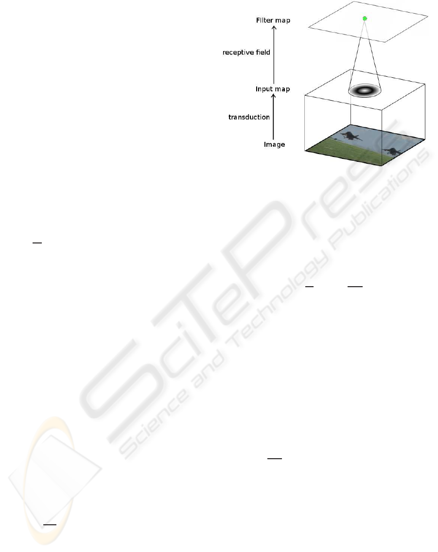
Figure 1: Pixel values of an input image are transformed
into spike trains (transduction operation) by Input map neu-
rons. Filter map neurons are connected to Input map neu-
rons through their receptive field (called connection mask).
Neurons of the Filter map realize a temporal integration of
spikes sent by Input map neurons to produce the neural fil-
tering result.
interval
ˆ
t
i
defined by:
ˆ
t
i
= −
1
λ
i
ln

1−
λ
i
ϑ
KL
i

(3)
This neuron produces a periodic spikes train s
i
(t):
s
i
(t) =
∞
∑
f=1
δ(t − f
ˆ
t
i
) (4)
where δ(.) is the Dirac distribution, with δ(x) = 0 for
x 6= 0 and
R
+∞
−∞
δ(x)dx = 1.
2.2 Neural Filtering
The neurons of Filter map integrate spike trains sent
by Input map neurons. For a given neuron j of Filter
map, the membrane potential V
j
is determined by:
dV
j
dt
= −λ
j
V
j
(t) +
∑
i∈P
j
w
ij
s
i
(t) (5)
where P
j
is the set of Input map neurons connected
to the neuron j and w
ij
is the connection weight be-
tween neurons i and j. The influence of Input map
spikes described in Equation (5) is known as instanta-
neous synaptic interaction. Thus, the evolution of the
membrane potential V
j
can be express as:
V
j
(t) =
P
j
∑
i=1
w
ij
∞
∑
f=1
e
−λ
j
(t− f
ˆ
t
i
)
H(t, f
ˆ
t
i
) (6)
where H(t, f
ˆ
t
i
) is the Heaviside function, with
H(t, f
ˆ
t
i
) = 1 if t > f
ˆ
t
i
and 0 otherwise.
IJCCI 2009 - International Joint Conference on Computational Intelligence
468

Neurons of Filter map are connected to Input map
neurons through a connection mask (Wolff et al.,
1999), which explicits the weight value of each con-
nection. A connection mask defines a type of generic
receptive field (see Figure 1) and the same connection
mask is shared by all the Filter map neurons.
The spikes produced by Filter map neurons are in-
terpreted to construct the resulting image filtering. A
gray level value l is associated to each Filter map neu-
ron, which represent the normalized discharge rate,
and this value is computed as:
l(x, y) =
NS(x,y)
MAX
x,y
(NS)
× depth (7)
where NS(x,y) is the number of spikes emitted by
the neuron at the location (x, y) and depth is the out-
put image depth. The resulting image displays a gray
level value l = 0 for neurons that have not emitted a
spike. For the other neurons, gray values code for the
number of spike emitted.
2.3 Computational Cost
The computational cost of a simulation of this spiking
neuron network is implementation-dependent. The
network described in this study is implemented with
an asynchronous approach: a simulated time step ∆t
is defined and for each ∆t the active neurons (i.e. neu-
rons which receive inputs) are updated. The param-
eter ∆t must be carefully set as it has a direct influ-
ence on the precision of simulation and the compu-
tational cost of the algorithm: increasing the preci-
sion is made at the expense of the computational cost.
Here, the chosen value of ∆t (0.1 millisecond) is very
small compared to the highest discharge rate observed
during simulations (≈10 Hz) ensuring that results are
precises and reproducibles.
The overall computation cost can be expressed as
the sum of the cost of updates and the cost of spikes
propagation:
c
u
×
A
∆t
+ c
p
× F × (NxM) × P
j
(8)
The cost of updates depends on c
u
(the cost of updat-
ing one neuron), the average number A of active neu-
rons (only neurons which receive spike are process)
and ∆t. The cost of propagating spikes is a function
of c
p
(the cost of propagating one spike), the mean
discharge rate F, the number of neurons (here, it is
the image size, NxM) and P
j
the number of output
connections.
In the proposed network, the cost of updates for
Input map neurons can be discarded as the inter-spike
interval is constant: it can be computed off-line and
stored in a LUT. The propagation cost of spikes emit-
ted by Filter map neurons is also negligible: they are
only stored for building the resulting image. Hence,
the computational cost is strongly related to the num-
ber of spikes emitted by Input map neurons and this
number is data-dependent. In the worst case, the
computational cost of neural filtering is in O(NxM),
which is comparable to the cost of image convolution
(in the case of non-separable filter).
3 RESULTS
In order to explore the boundaries recovery ability of
the neural filtering method, we propose to compare it
to the performances made by the DOG convolution in
the same conditions. The DOG impulse response is
defined as:
DOG(x,y) =
1
2πσ
2
1
e
−
x
2
+y
2
2σ
2
1
−
1
2πσ
2
2
e
−
x
2
+y
2
2σ
2
2
(9)
For the convolutional DOG method, the value of
σ
1
is set to 1 and the value of σ
2
is set to 3.
For the neural filtering method, the weight values
of the connection mask are computed with the DOG
impulse response defined in Equation (9) (with the
same value as above : σ
1
= 1 and σ
2
= 3) and are nor-
malized between −w
max
and w
max
. The value of the
spiking neuron network parameters are w
max
= 0.4,
λ
i
= 0.005 and λ
j
= 0.001.
3.1 Methodology of the Validation
The validation of the neural-based method is divided
in two main phases. First, a validation on synthetic
images is done in order to compare the noise resis-
tance ability of this algorithm versus the convolu-
tional one. Then, a study on natural images is per-
formed to study the edges retrieval ability of the neu-
ral method on images corrupted by ”natural” noise.
In the first phase, three different kind of noises
were used to corrupt the original image: the Gaussian
noise, the Poisson noise and the salt and pepper. For
each type, various levels of noise are applied. As the
goal of this validation is to study edges preservation
ability of both methods, the Sobel filtered original im-
age is compared to image resulting from the following
process: the original image is corrupted with a given
noise, it is then filtered with the neural method, even-
tually a Sobel filter is applied and finally a threshold-
ing. The same comparison is done for the convolu-
tional filtering. An example of each step of the pro-
cess can be seen on Figure 2, which present the result
on Gaussian noise.
DIFFERENCE OF GAUSSIANS TYPE NEURAL IMAGE FILTERING WITH SPIKING NEURONS
469

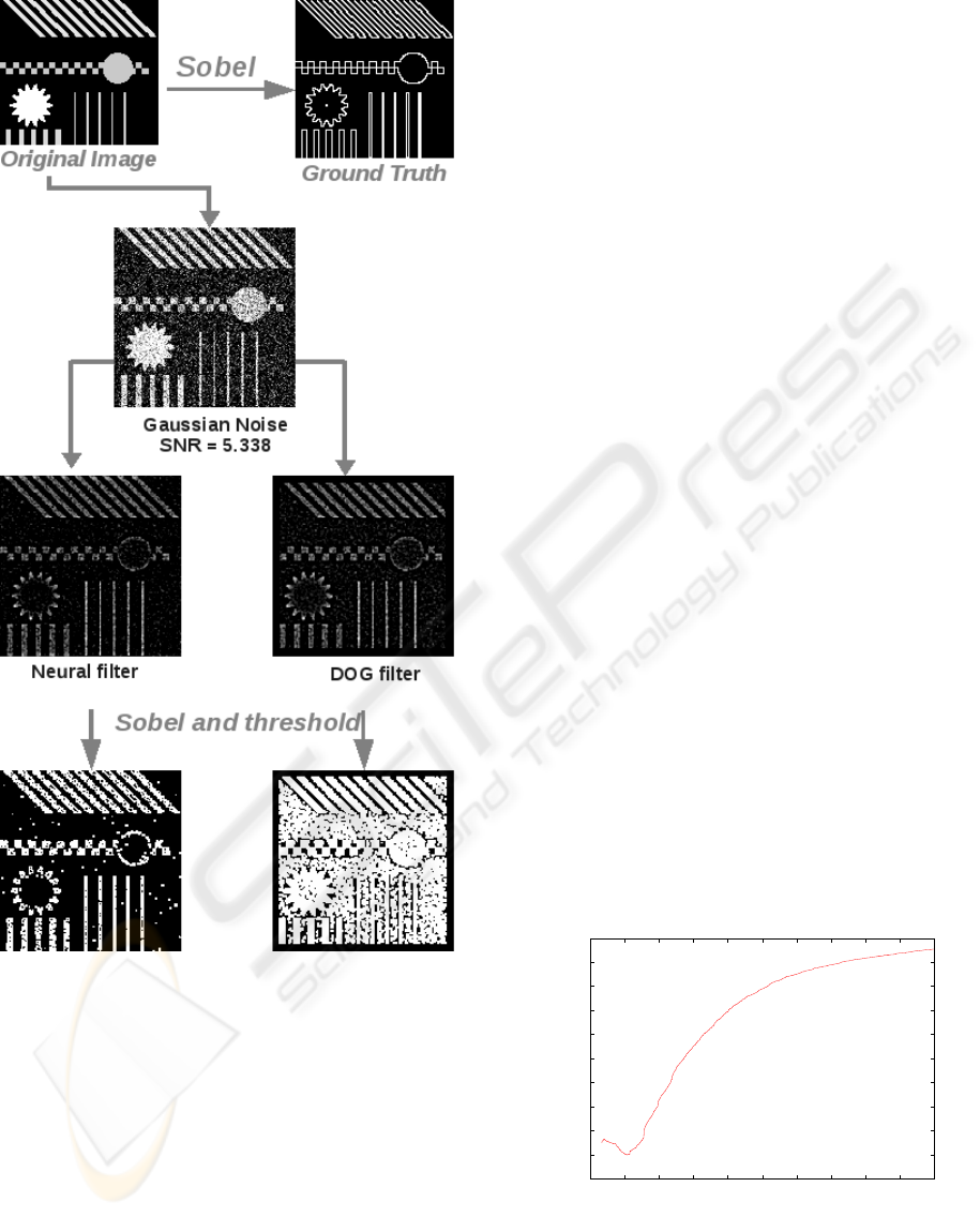
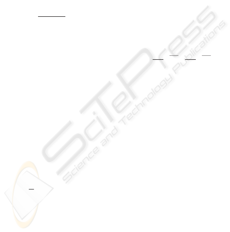
Figure 2: This figure represents the whole process of vali-
dation made on a synthetic image.
It is important to remind that the Sobel operator
computes an approximation of the gradient of image
intensity function and thus gives edges with various
gray levels depending on gradient values. One can
thus consider that the higher the gray value is, the
stronger the edge is. But as the information encod-
ing is different for neural and convolutional methods,
a direct comparison is not possible. In order to com-
pare fairly both methods, it has been decided to do a
binarization of the image resulting of the Sobel filter
and to consider that all the edges had the same impor-
tance. This approach allowed to study details preser-
vation, resistance to artifacts created by noise and it
is independent from the information coding used in
neural method or in convolutional one. Therefore, a
threshold was applied on resulting Sobel filtered im-
ages: all values strictly higher than 0 were preserved
in giving them the value 255. The calculation of the
performance of both algorithms was done using the
Mean Squared Error estimator, considering that the
ground truth is the binary result of the Sobel applied
on original image.
It has to be noticed that we deliberately decided
not to calculate SNR (Signal to Noise Ratio) on re-
sulting images since the aim here is edges determina-
tion and preservation and both convolutional and neu-
ral algorithms do not process a good filtering in term
of original image retrieval.
On a second time, we decided to perform the val-
idation of our method on natural images. Knowing
that natural images are usually corrupted by noise,
edges attenuation, blur in some cases, the aim here
was to study the behaviour of the neural method on
this kind of images and to compare it to convolutional
filtering. Due to the difficulty of finding realistic esti-
mators in such cases, a visual estimation of the preser-
vation and enhancement of edges was performed.
3.2 Experimental Results on Synthetic
Images
The experimental validation process explained in the
previous section is done on a 256x256 pixels synthetic
8-bit grayscale image (presented on the top of the Fig-
ure 2). The chosen parameter values for convolutional
and neural filtering are described in Sect. 3. Figure 4
shows the results obtained for the different noise type
(Gaussian, Poisson and salt and pepper).
8000
10000
12000
14000
16000
18000
20000
22000
24000
26000
28000
0 100 200 300 400 500 600 700 800 900 1000
MSE
simulated time
Evolution of MSE during neural simulation
Figure 3: The MSE is computed for each time step during a
neural simulation (here for Gaussian noise with σ = 85).
These data are processed to determine the “worst” and
“best” values for neural filtering.
IJCCI 2009 - International Joint Conference on Computational Intelligence
470

5000
10000
15000
20000
25000
30000
35000
40000
45000
50000
0 20 40 60 80 100 120 140
MSE
σ
Gaussian noise
convolution
neuronal
best neuronal
worst neuronal
0 20 40 60 80 100 120 140
mean
Poisson noise
convolution
neuronal
best neuronal
worst neuronal
5 10 15 20 25 30 35 40 45 50
% of flipped pixels
Salt and pepper noise
convolution
neuronal
best neuronal
worst neuronal
Figure 4: Evaluation of contour preservation for Gaussian (left), Poisson (center) and salt and pepper noises (right). The
neural-based algorithm outperform the convolution one.
The quality of the results produced by the neural-
based method are dependent from the spiking neuron
network simulation time. The number of simulated
time step ∆t is a parameter of this method. Figure 3
shows the evolution of the measured MSE for simu-
lated time step ∆t ∈ [0;1000]. One can notice that the
curve seems to reach its minimum in few steps (gen-
erally between 80 and 120 time steps). After that the
process seems to degrade the image in term of edges
preservation. Hence, for each experiment (i.e. each
noise level) the MSE is computed for each simulated
time step ∆t. The worst and the best score are then de-
termined and these values are referred on the Figure 4
as “worst neuronal” and “best neuronal”. On these
figures, an MSE score is represented for an empiri-
cally determined stopping criteria (∆t = 115), which
is called “neuronal”. As one can see in Figure 4 neu-
ral filtering is always better in term of MSE measure
for contour preservation, even for “worst neuron”.
A visual validation has also been made to check
that even visually the results were better for neural-
based filtering. For an example of such denoised im-
ages, see Figure 2.
3.3 Experimental Results on Natural
Images
As mentioned before, the evaluation were also per-
formed on natural image.
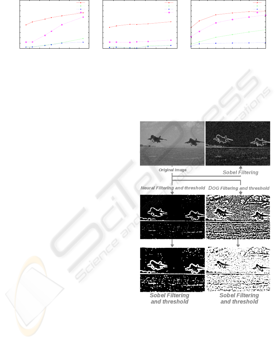
A Sobel filter is applied on a natural image and
is compared to the natural image filtered with DOG
convolution or neural filter and a Sobel filter.
This visual method is used to study the edges
preservation and enhancement. An example of such
a process is given in Figure 5.
It has to be noticed that due to differences in in-
formation coding and so as to compare fairly both
methods, a threshold has been applied on DOG and
neural filtered images for visual inspection. The same
threshold is applied on images for visual inspection
after the application of the Sobel operator as ex-
plained in the previous section.
As we can see here, neural filter seems to be less
influenced by noise level in the original image than
the DOG filter and seems to retrieve better the princi-
pal edges of the image.
Figure 5: This figure represents an example of the valida-
tion process made on natural images. A Sobel filter is first
applied to the natural image and is compared to the result of
the filtering of the original image with a Neural (or DOG)
filter and a Sobel one.
DIFFERENCE OF GAUSSIANS TYPE NEURAL IMAGE FILTERING WITH SPIKING NEURONS
471

4 CONCLUSIONS
In this paper we detailed a novel filtering algorithm
based on an spiking neurons network. The pixel val-
ues of the input image are transformed into spike
trains on an Input map. The generated spike train are
processed by a Filter map which realize a temporal
integration of these spike trains. The result of this in-
tegration is the neural filtered result.
For DOG filtering, the neural-based method is
tested on synthetic and natural images and outper-
form the classical DOG convolution in terms of edges
preservation and retrieval in noisy images. It has been
shown that for other filtering algorithms based on an
iterative process, the question of the stopping crite-
ria determination is crucial. Therefore the presented
results always mentioned the worst and the best ob-
tained results.
REFERENCES
Abbott, L. (1999). Lapicque’s introduction of the integrate-
and-fire model neuron (1907). Brain Research Bul-
letin, 50(5-6):303–304.
Ahrns, I. and Neumann, H. (1999). Space-variant dynamic
neural fields for visual attention. In Int. Conf. on Com-
puter Vision and Pattern Recognition (CVPR), vol-
ume 2, page 318. IEEE Computer Society.
Chevallier, S. and Tarroux, P. (2008). Covert attention with
a spiking neural network. In Gasteratos, A., Vincze,
M., and Tsotsos, J., editors, Int. Conf. on Computer
Vision Systems (ICVS), volume 5008 of Lecture Notes
in Computer Science, pages 56–65. Springer.
Chevallier, S., Tarroux, P., and Paugam-Moisy, H. (2006).
Saliency extraction with a distributed spiking neural
network. In Verleysen, M., editor, European Sympo-
sium on Artificial Neural Networks (ESANN), pages
209–214, Bruges, Belgium.
de Brecht, M. and Saiki, J. (2006). A neural network imple-
mentation of a saliency map model. Neural Networks,
19(10):1467–1474.
Enroth-Cugell, C. and Robson, J. (1966). The contrast sen-
sitivity of retinal ganglion cells of the cat. Journal of
Physiology, 187(3):517–552.
Fix, J., Vitay, J., and Rougier, N. (2007). A distributed com-
putational model of spatial memory anticipation dur-
ing a visual search task. In Anticipatory Behavior in
Adaptive Learning Systems, Lecture Notes in Artifi-
cial Intelligence, pages 170–188.
Fouquier, G., Atif, J., and Bloch, I. (2008). Incorporating a
pre-attention mechanism in fuzzy attribute graphs for
sequential image segmentation. In Int. Conf. on Infor-
mation Processing and Management of Uncertainty in
Knowledge-Based Systems (IPMU), pages 840–847.
Frintrop, S., Jensfelt, P., and Christensen, H. (2006). Atten-
tional landmark selection for visual slam. In Int. Conf.
on Intelligent Robots and Systems, pages 2582–2587.
IEEE Computer Society.
Gerstner, W. and Kistler, W. (2002). Spiking Neuron Mod-
els: Single Neurons, Population, Plasticity. Cam-
bridge University Press, New York, NY, USA.
Itti, L., Koch, C., and Niebur, E. (1998). A model of
saliency-based visual attention for rapid scene anal-
ysis. IEEE Transactions on Pattern Analysis and Ma-
chine Intelligence (PAMI), 20(11):1254–1259.
Itti, L., Rees, G., and Tsotsos, J., editors (2005). Neurobi-
ology of Attention. Elsevier, San Diego, USA.
K¨onig, P., Engel, A., and Singer, W. (1996). Integrator or
coincidence detector? the role of the cortical neuron
revisited. Trends in Neurosciences, 19(4):130–137.
Maass, W. (1997). Networks of spiking neurons: the third
generation of neural network models. Neural Net-
works, 10:1659–1671.
Maillard, M., Gapenne, O., Gaussier, P., and Hafemeister,
L. (2005). Perception as a dynamical sensori-motor
attraction basin. In Advances in Artificial Life, volume
3630 of Lecture Notes in Computer Science, pages
37–46. Springer.
Michalke, T., Fritsch, J., and Goerick, C. (2008). Enhanc-
ing robustness of a saliency-based attention system
for driver assistance. In Int. Conf. on Computer Vi-
sion Systems (ICVS), volume 5008 of Lecture Notes
in Computer Science, pages 43–55. Springer.
Tsotsos, J. (1989). The complexity of perceptual search
tasks. In Int. Joint Conf. on Artificial Intelligence (IJ-
CAI), pages 1571–1577. AAAI, Detroit, USA.
Tsotsos, J. (1990). Analysing vision at the complexity level.
Behavioral and Brain Sciences, 13:423–469.
Vitay, J., Rougier, N., and Alexandre, F. (2005). A
distributed model of spatial visual attention. In
Biomimetic Neural Learning for Intelligent Robots,
Lecture Notes in Artificial Intelligence, pages 54–72.
Springer.
Wolff, C., Hartmann, G., and Ruckert, U. (1999).
ParSPIKE-a parallel DSP-accelerator for dynamic
simulation of large spiking neural networks. In Int.
Conf. on Microelectronics for Neural, Fuzzy and Bio-
Inspired Systems (MicroNeuro), pages 324–331. IEEE
Computer Society.
IJCCI 2009 - International Joint Conference on Computational Intelligence
472