
BRAIN COMPUTER INTERFACE
Application of an Adaptive Bi-stage Classifier based on RBF-HMM
Jos´e Luis Mart´ınez P´erez and Antonio Barrientos Cruz
Grupo de Rob´otica y Cibern´etica, Universidad Polit´ecnica de Madrid, C/Jos´e Gutierrez Abascal 2, Madrid, Spain
Keywords:
Electroencephalography, Brain computer interface, Linear discriminant analysis, Spectral analysis, Biomedi-
cal signal detection, Pattern recognition.
Abstract:
Brain Computer Interface is an emerging technology that allows new output paths to communicate the users
intentions without the use of normal output paths, such as muscles or nerves. In order to obtain their objective,
BCI devices make use of classifiers which translate inputs from the users brain signals into commands for
external devices. This paper describes an adaptive bi-stage classifier. The first stage is based on Radial Basis
Function neural networks, which provides sequences of pre-assignations to the second stage, that it is based
on three different Hidden Markov Models, each one trained with pre-assignation sequences from the cognitive
activities between classifying. The segment of EEG signal is assigned to the HMMwith the highest probability
of generating the pre-assignation sequence.
The algorithm is tested with real samples of electroencephalografic signal, from five healthy volunteers using
the cross-validation method. The results allow to conclude that it is possible to implement this algorithm in an
on-line BCI device. The results also shown the huge dependency of the percentage of the correct classification
from the user and the setup parameters of the classifier.
1 INTRODUCTION
Since that Dr. Hans Berger discovered the electrical
nature of the brain, it has been considered the possi-
bility to communicate persons with external devices
only through the use of the brain waves (Vidal, 1973).
Brain Computer Interface technology (Wolpaw,
J.R.; et al., 2000) is aimed at communicating with
persons using external computerized devices via the
electroencephalographic signal as the primary com-
mand source (Birbaumer, N; et al., 2000); in the first
international meeting for BCI technology it was esta-
blished that BCI “must not depend on the brain’s nor-
mal output pathways of peripheral nerves and mus-
cles” (Wolpaw, J. R.; et al., 2002). The primary uses
of this technology are to benefit persons with block-
ing diseases, such as: Amiotrophic Lateral Sclerosis
(ALS), brainstem stroke, or cerebral palsy; or persons
whom have suffered some kind of traumatic accident
like for example paraplegic (E. Donchin and K. M.
Spencer and R. Wijesinghe, 2000). In order to control
an external device using thoughts, it is necessary to
associate some mental patterns to device commands.
Therefore, an algorithm that detects, acquires, filters,
and classifies the electroencephalographic signal is
required (Kostov, A.; Polak, M., 2000) (Pfurtscheller
et al., 2000b). Actually different types of classifica-
tions can be established for BCI technology, from the
physiologic point of view BCI devices can be clas-
sified in exogenous and endogenous. The devices in
the first group provide some kind of stimuli to the user
and they analyze the user’s responds to them, exam-
ples of this class are devices based on visual evoked
potential or P300 (E. Donchin and K. M. Spencer and
R. Wijesinghe, 2000). On the contrary, the endoge-
nous devices does not depend on the user’s respond to
external stimuli, they base their operationin the detec-
tion and recognition of brain-wave patterns controlled
autonomously by the user, examples of this class are
devices based on the desynchronization and synchro-
nization of µ and β rhythms (Wolpaw, J. R.; et al.,
2002), (Pfurtscheller et al., 2000a), (Pineda, J.A. et
al., 2003).
In this paper is presented an endogenous classi-
fier composed of two adaptive stages. In the first
stage a Radial Basis Function neural network (Ripley,
2000) performs a pre-classification of the segment of
EEG input signal and provides a pre-assignation se-
quence of data to the second stage. In this second
stage is computed the generation probability of the in-
13
Luis Martínez Pérez J. and Barrientos Cruz A. (2010).
BRAIN COMPUTER INTERFACE - Application of an Adaptive Bi-stage Classifier based on RBF-HMM.
In Proceedings of the Third International Conference on Biomedical Electronics and Devices, pages 13-20
DOI: 10.5220/0002692700130020
Copyright
c
SciTePress
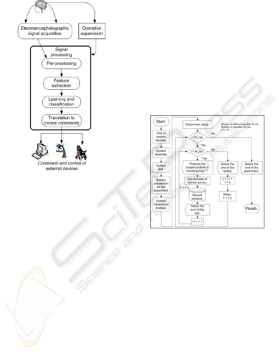
Figure 1: Block diagram of a BCI device.
put sequence by three different Hidden Markov Mod-
els, each one had been previously trained with data
sequences from the different cognitive activities be-
tween classifying.
The content of this paper is as follows:
• Section 2 describes the experimental procedure,
the cognitive activities or mental tasks, and the
equipment to develop the experiment.
• Section 3 presents the proposed two-stage classi-
fier and describes the algorithms employed in it
for training and operation.
• Section 4 presents the results obtained from each
volunteer.
• Section 5 analyzes the previous results.
• And finally section 6 is devoted to making conclu-
sions.
2 EXPERIMENTAL PROCEDURE
The tests described below were carried out on five
healthy male subjects, one of whom had been trained
before but the other four of whom were novices in the
use of the system.
In order to facilitate the mental concentration ne-
cessary for the proposed activities, the experiments
were carried out in a room with a low noise level
and under controlled environmental conditions. For
instance, all electronic equipment external to the ex-
periment and unrelated to the subject were switched
off in order to avoid electromagnetic artifacts. The
experiments were carry out between 10:00 a.m. and
14:00 p.m. The subjects were directed to sit down 50
cm from the screen of the acquisition system monitor,
and with their hands in a visible position. The super-
visor of the experiment ensured the correct enactment
of this process.
2.1 Flow of Activities in the
Experimental Process
The experimental process is shown in Figure 2.
Figure 2: Diagram of the experiment carried out.
System Devices Test. The correct battery level and
correct state of the electrodes were checked.
System Assembly. Device connections: superfi-
cial electrodes (Grass Au-Cu), battery, bio-amplifier
(g.BSamp by g.tec), acquisition signal card (PCI-
MIO-16/E-4 by National Instrument), computer.
System Test. The correct operation of the whole
system was verified. To minimize noise from the
electrical network the Notch filter (50Hz) of the bio-
amplifier was switched on.
Subject Preparation for the Experiment.
Electrodes were applied to the subject’s head.
Electrode impedance ≤ 4KOhms.
System Initialization and Setup. The data register
was verified. The signal evolution was monitored; it
was imperative that a very low component of 50 Hz
appeared within the spectrogram.
BIODEVICES 2010 - International Conference on Biomedical Electronics and Devices
14
Experiment Setup. The experiment supervisor set
up the number of replicationsN
rep
= 10, and the quan-
tity of different mentalactivities. The durationof each
trial was t = 7s, and the acquisition frequency was
f
s
= 384Hz. The system suggested that the subject
think about the proposed mental activity. A short re-
laxation period was allowed at the end of each trial;
between replications the relax time is t = 7s.
2.2 Electrode Position
Electrodes were placed in the central zone of the
skull, next to C3 and C4 (Penny, W. D.; et al., 2000),
and two pairs of electrodes were placed in front of and
behind the Rolandic sulcus. This zone has the highest
discriminatory power and receives signals from mo-
tor and sensory areas of the brain (Birbaumer, N; et
al., 2000) (Neuper, C.; et al., 2001). A reference elec-
trode was placed on the right mastoid and two more
electrodes were placed near the corners of the eyes to
register blinking.
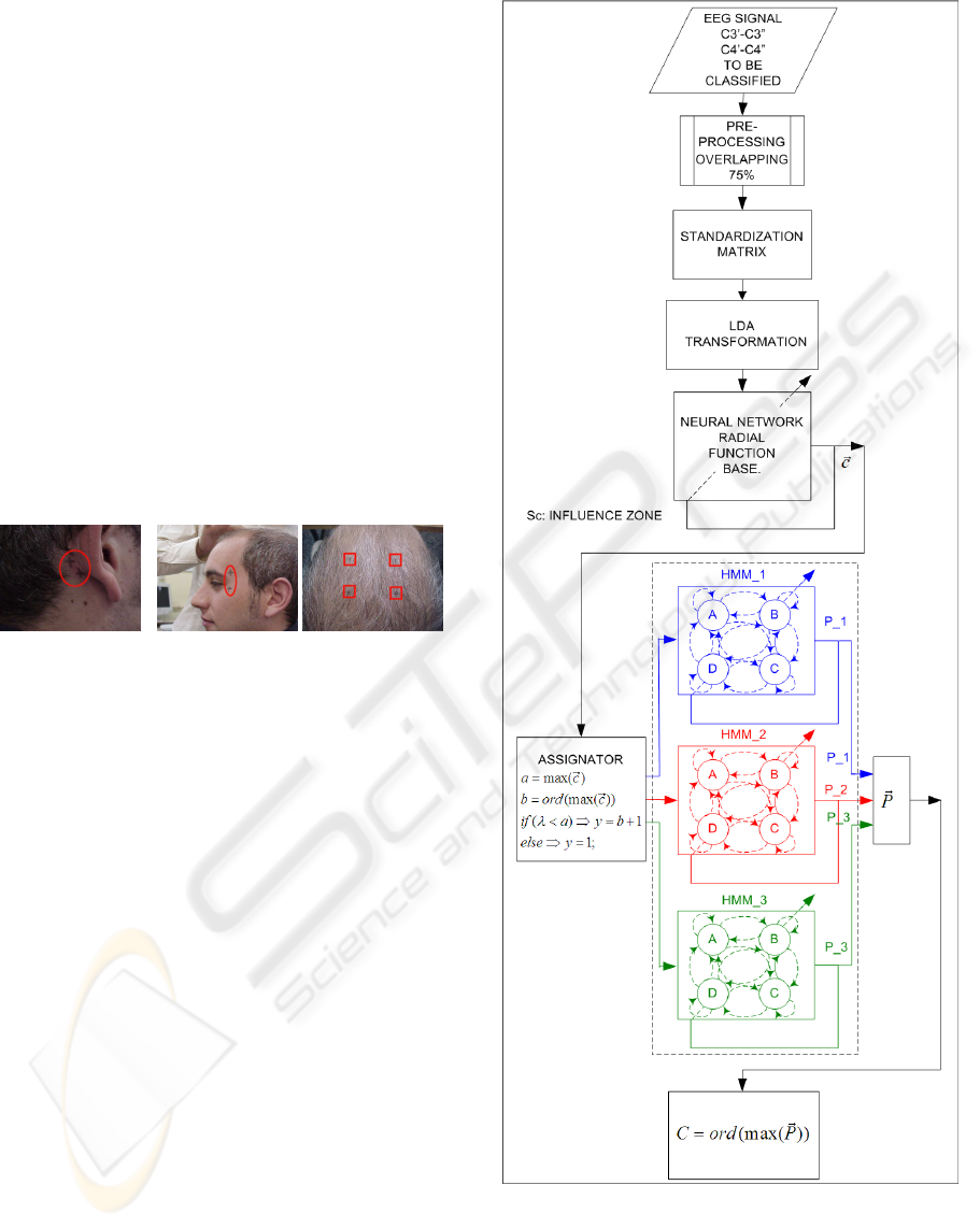
Figure 3: Electrode placement.
2.3 Description of Cognitive Activities
The experiment supervisor asked the subject to figure
out the following mental activities; tasks that were
used to differentiate between cerebral patterns (Ne-
uper, C.; et al., 2001):
Activity A. Mathematical task. Recursive subtraction
of a prime number, i.e. 7, from a large quantity, i.e.
3.000.000.
Activity B. Movement task. The subject imagines
moving their limbs or hands, but without actually do-
ing so. It is movement imagery.
Activity C. Relax. The subject relaxes.
3 DESCRIPTION OF THE
CLASSIFIER
3.1 Introduction
In Figure 4 is shown the block diagram of the algo-
rithm for the proposed classifier.
In it can be appreciated how the classification of
the considered segment of the EEG signal is obtained
after the evaluation of the probability generation of
Figure 4: Block diagram of the classifier.
the pre-assignation sequence provided by three Hid-
den Markov Models.
There are as many Hidden Markov Models as cog-
nitive activities to be considered for the classification,
BRAIN COMPUTER INTERFACE - Application of an Adaptive Bi-stage Classifier based on RBF-HMM
15
each model is trained with pre-assignation sequences
of data of the cognitive activity associated to it.
The pre-assignation sequence of data are provided
by a neural network, which inputs are the vectors of
features obtained after the preprocessing of the seg-
ment of EEG signal, as it is described in the following
subsections.
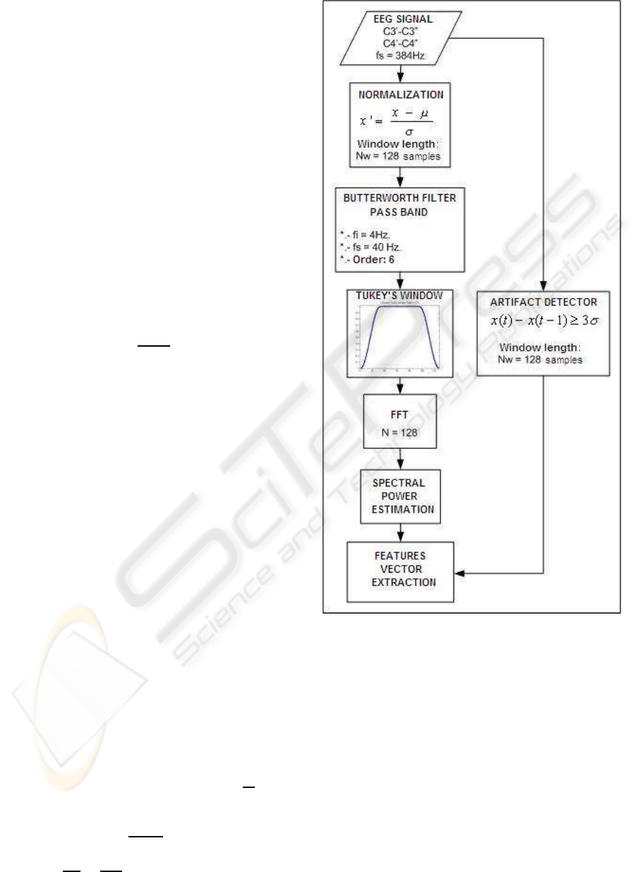
3.2 Preprocessing
On Figure 5 is depicted the operations associated to
the preprocessing phase.
In a first step the EEG signal coming from both
electroencephalographic channels C3’-C3” and C4’-
C4” are sampled and quantified at f
s
= 384Hz.
In the next step the samples are bundled in pack-
age of N
w
= 128 samples, it is equivalent to T
w
=
1/3s. Each group of samples is normalized, in order
to obtain homogenous groups of transformed samples
with zero mean value and unity as standard deviation.
x
′
i
=
x
i
− µ
σ
(1)
This transformation does not affect the frequency
properties of the signal, but allows the comparison of
groups of samples in the same session or between ses-
sions, it avoids that changes in the impedance of the
electrodes or skin conductivity affect the next proce-
dures.
After this the samples are processed by a pass
band Butterworth filter of order n = 6, with lower
and higher frequencies of f
1
= 4Hz and f
2
= 40Hz
(Proakis and Manolakis, 1997); frequencies outside
this band are not common in sane conscious users.
In the next step the filtered samples are convoluted
with a Tukey’s window of length N = 128, this ate-
nuates the leakage effect associated to the package
procedure, see Figure 6. Previous studies allow to
conclude that the convolution of the signal with this
kind of window increase the discrimination capabil-
ity that the one obtained with other kind of windows
as for example: rectangular, triangular, Blackman’s,
Hamming’s, Hanning’s or Kaiser’s (Martinez, J.L.;
Barrientos, A., 2006).
After the convolution, the Fast Fourier Transform,
eq.2, is applied in order to obtain the spectral power
estimation, eq.3; the obtained frequency resolution is
in eq.4.
X(k) =
N
∑
j=1
x( j)w
( j− 1)(k−1)
N
; w
N
= e
−
2πi
N
(2)
P(k) =
X(k)
2
N
(3)
∆f =
f
s
N
w
=
384
128
= 3Hz (4)
Figure 5: Block diagram for the preprocessing phase.
After the estimation of each frequency band, it is
computed the vector of features consideringthe power
average of the involved bands as it is shown on Table
1.
In case of presence of artifacts the algorithm de-
tects them and during the learning phase it substitutes
its value by the average value of the samples in that
package, if the artifacts are detected in the on-line
phase, it instructs the classifier to discard that group
of samples.
A group of samples is considered with artifacts
if one sample differs more than three standard de-
viations from the previous one.
BIODEVICES 2010 - International Conference on Biomedical Electronics and Devices
16
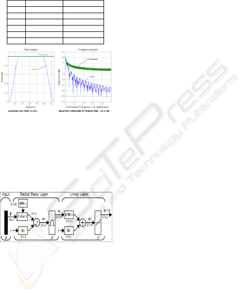
Table 1: Feature vector.
Index Denomination. Frequency (Hz).
1 θ. 6 - 8
2 α
1
. 9 - 11
3 α2. 12 - 14
4 β
1
. 15 - 20
5 β
2
. 21 - 29
6 β
3
. 30 - 38
Figure 6: Frequency leakage effect.
3.3 Training of the Neural Network
The considered neural network is the type of Radial
Function Basis. Thistype of neuralnetwork is charac-
terized by the learning of the position of the samples
in the training set and by the interpolation capability
between them (Ripley, 2000).
In Figure 7 is represented the architecture of this
type of neural network.
Figure 7: Architecture of the RBF neural network.
From previous studies it has been concluded that
this type of neural network behaves better than other
types of neural networks, as for example Multi-Layer
Perceptrons or Probabilistic Neural Networks (Mar-
tinez, J.L.; Barrientos, A., 2008).
The activation function is:
radbas(x) = e
−x
2
; x = (~w−~p) ∗ S
c
(5)
In where ~w and S
c
are respectively the weights and
influence zone constant of each neuron, and ~p is the
position of the considered sample.
During the learning phase the neurons of the hid-
den layer learn the position of the samples of the
learning set, ~w; during the test phase when a new sam-
ple~p is presented, it is computed the distancebetween
the sample and the learned positions, the nearest neu-
rons to the samplewill proportionate higheractivation
values than the rest of the neurons.
For the learning process are considered vectors of
features from the EEG signal, acquired when the user
was performing one of the different cognitive activi-
ties considered for the classification. The learning set
is composed by the 75% of all the sample set, and the
other 25% is considered for validation. After the de-
termination of the learning and validation sets, the in-
put vectors to the neural network are normalized, and
with LDA technique is reduced their dimensionality
projecting the original input vectorsin the direction of
the highest discrimination capability (Martinez, J.L.;
Barrientos, A., 2007).
In order to minimize the over-learning effect, the
RBF learning process allows a dynamic growth of the
number of neurons in the hidden layer. In the out-
put layer are considered as many linear neurons as
cognitive activities between discriminate. Finally in
the assignation block on Figures 4, it is weighted the
output vector of the neural network and it assigns the
input vector to the activity with highest output value
provided it is higher than a threshold λ, on the con-
trary if the value is lower than λ, the input vector is
labeled as unclassified.
On operation, once the neuronal network has been
trained, when a new vector is presented the cogni-
tive activity, with samples nearer to it, will provide
a higher activation level, and the corresponding out-
put will have a higher value than the others cognitive
activities.
3.4 Description of Hidden Markov
Models
A Hidden Markov Model is a double stochastic sta-
tistical model, it consists of a Markov process with
unknown and non-observable parameters, and a ob-
served model which parameters depend stochastically
from the hidden states. A stochastic processis called a
Markovian process if the future does not depend from
the past, onlyfrom the known present; consideringthe
stochastic variable q(t − 1) the transition probability
in the instant t is defined as P(q
t
= σ
t
|q
t−1
= σ
t−1
). A
Markov chain is formally defined with the pair (Q,A),
where Q = {1,2, ..., N} are the possible estates of the
chain and A = [a
ij
] is the transition matrix of the
model, with the constrains:
BRAIN COMPUTER INTERFACE - Application of an Adaptive Bi-stage Classifier based on RBF-HMM
17
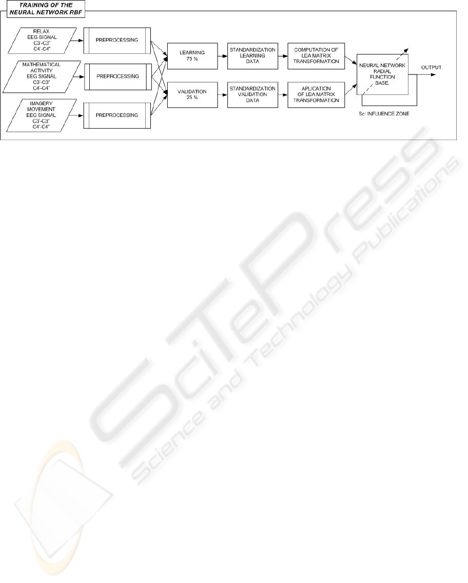
Figure 8: Training of the RBF neural network.
0 ≤ a
ij
≤ 1; 1 ≤ i, j ≤ N (6)
N
∑
j=1
a
ij
= 1; 1 ≤ i ≤ N (7)
The transition and emission probabilities depends
from the actual estate and no from the former estates.
P(q
t
= j|q
t−1
= i,q
t−2
= k,...) = (8)
= P(q
t
= j|q
t−1
= i) = a
ij
(t)
Formally a discrete HMM of first grade is defined
by the 5-tuple: λ = {Z,Q,A,B, π}, in where:
• Z = {V
1
,V
2
,...,V
M
} is the alphabet or discrete set
of M symbols.
• Q = {1,2,...,N} is the set of N finite estates.
• A = [a
ij
] is the transition matrix of the model.
• B = (b
j
(Q
t
))
NxM
is the matrix of emission sym-
bols, also known as observation matrix.
• π = (π
1
,π
2
,...,π
N
) is the prior probability vector
of the initial estate.
The parameters of a HMM are λ = {A,B,π}.
There are three types of canonic problems associated
to HMM (Rabiner, 1989)(Rabiner and Juang, 1986):
1. Given the parameters of the model, obtain the
probability of a particular output sequence. This
problem is solved through a forward-backwards
algorithm.
2. Given the parameters of the model, find the most
probable sequence of hidden estates, that could
generate the given output sequence. This problem
is solved through the use of Viterbi algorithm.
3. Given an output sequence, find the parameters of
the HMM. This problem is solved through the use
of Baum-Welch algorithm.
The HMM have been applied specially in speech
recognition an generally in the recognition of tempo-
ral sequences, hand written, gestures, and bioinfor-
matics (Rabiner and Juang, 1986).
3.5 Training of the Hidden Markov
Models
The HMM’s are trained with sequences of pre-
assignations coming from the EEG samples, as it is
shown in the Figure 9.
For each cognitive activity a particular HMM,
with the following characteristics, is trained:
• Number of hidden estates: 4.
• Number of different observable objects: 4
In the training phase, chains of nine pre-
assignations were used. In a previous experiment
with synthetic samples, it was concluded that for the
proposed architecture of Hidden Markov Models the
highest percentage of correct classifications were ob-
tained with chains of nine elements.
After the training or solution of the third canonic
problem, the probability matrices of state transitions
and observation matrices are determined. The Viterbi
algorithm is used in order to determine the probability
that a model generates the proposed sequence.
4 RESULTS
In order to test the behavior of the proposed algo-
rithm, the influence of the threshold assignation pa-
rameter (λ), and the influence zone of the neuron (S
c
),
the EEG samples of the session tests from the volun-
teers were used as follows:
4.1 Evaluation of the Learning
Capability
With a subset of 75% of the all EEG samples the al-
gorithm was trained with different λ and S
c
values:
BIODEVICES 2010 - International Conference on Biomedical Electronics and Devices
18
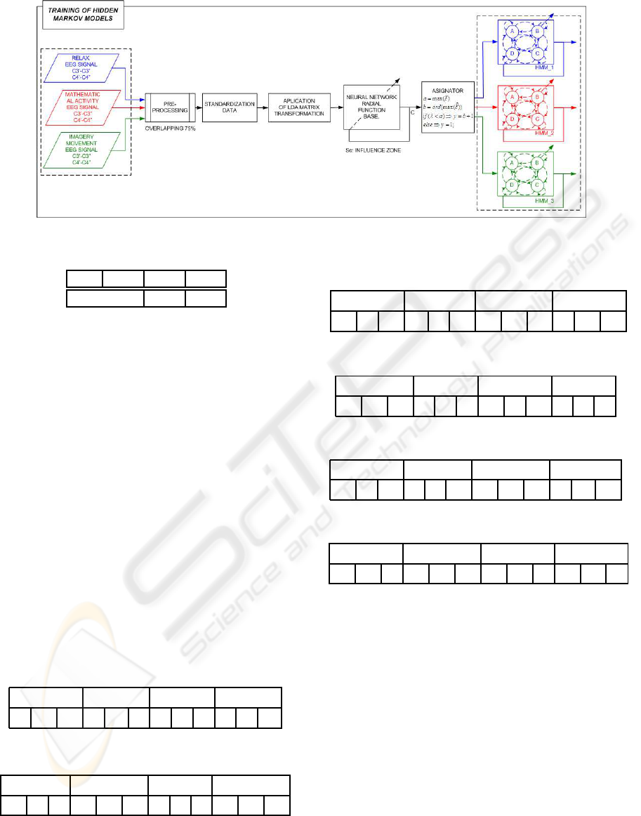
Figure 9: Training of the HMM.
λ = 0.55 0.65 0.8
S
c
= 0.5 0.95
These values have been fixed after a seek in wide
with the samples of the first volunteer.
After the learning, the same samples were pro-
cessed with the trained algorithm, and a comparison
between the results obtained with the algorithm and
the ones employed for the learning was done, in all
cases a 100% of correct classification has been ob-
tained.
4.2 Evaluation of the Generalization
Capability
After the good results obtained from the learning
phase, a cross-validation methodology is used to es-
timate the generalization capability. From the whole
ten sessions, nine are used for learningand one is used
for validation, the process is repeated ten times chang-
ing each time the session used for validation.
In the following tables are shown the results ob-
tained for each volunteer, considering the λ and S
c
parameters.
Table 2: Volunteer: Al01.
S
c
= 0.5 S
c
= 0.95 S
c
= 0.5 S
c
= 0.95
λ = 0.65 λ = 0.55 λ = 0.55 λ = 0.80
94 103 103 94 81 87 93 92 87 86 97 81
+4 +14 +14 +4 -10 -3 +3 +2 -3 -4 +8 -10
Table 3: Volunteer: Ro01.
S
c
= 0.5 S
c
= 0.95 S
c
= 0.5 S
c
= 0.95
λ = 0.65 λ = 0.55 λ = 0.55 λ = 0.80
103 97 92 118 109 118 97 87 86 117 106 110
+14 +8 +2 +31 +21 +31 +8 -3 -4 +30 +18 +22
For each combination, the process is replicated
three times. In the upper row it is shown the num-
ber of correct classifications. In the lower row it is
Table 4: Volunteer: Ja01.
S
c
= 0.5 S
c
= 0.95 S
c
= 0.5 S
c
= 0.95
λ = 0.65 λ = 0.55 λ = 0.55 λ = 0.80
106 97 110 87 90 107 99 106 107 98 108 99
+18 +8 +22 -3 0 +19 +10 +18 +19 +9 +20 +10
Table 5: Volunteer: Da01.
S
c
= 0.5 S
c
= 0.95 S
c
= 0.5 S
c
= 0.95
λ = 0.65 λ = 0.55 λ = 0.55 λ = 0.80
109 102 104 83 92 92 106 91 110 86 87 92
+21 +13 +15 -8 +2 +2 +18 +1 +22 -4 -3 +2
Table 6: Volunteer: Ra01.
S
c
= 0.5 S
c
= 0.95 S
c
= 0.5 S
c
= 0.95
λ = 0.65 λ = 0.55 λ = 0.55 λ = 0.80
106 97 110 87 90 107 99 106 107 91 76 99
+18 +8 +22 -3 0 +19 +10 +18 +19 +1 -15 +10
Table 7: Volunteer: Ra02.
S
c
= 0.5 S
c
= 0.95 S
c
= 0.5 S
c
= 0.95
λ = 0.65 λ = 0.55 λ = 0.55 λ = 0.80
102 102 98 102 107 114 103 105 96 116 99 98
+13 +13 +9 +13 +19 +26 +14 +16 +6 +29 +10 +9
shown the percentage of improvement against a naive
classifier.
5 DISCUSSION
From the results of the proposed classification algo-
rithm, it is observed that:
• The learning capability is better that the one
achieved only with the RBF neural network (Mar-
tinez, J.L.; Barrientos, A., 2008).
• From the analysis of the results of the replicas
it has been detected that the variability in the
percentage of correct classifications is caused by
the HMM’s, both in the learning and validation
phases. The sequences of pre-assignations pro-
BRAIN COMPUTER INTERFACE - Application of an Adaptive Bi-stage Classifier based on RBF-HMM
19

vided by the neural network were stable, but the
generation probabilities of the HMM’s changed in
each replica. In the learning phase the HMM’s
probabilities allowed a perfect classification, but
they were not maintained in the cross validation
phase; for this stage a lower percentage of correct
classification was obtained, as it is summarized in
the tables 2 to 7. But until in this case, almost in
all replicas, the cross-validation test results were
better than the ones hoped from a naive classifier.
• The values of correct classifications depend
highly from the user. There has not been identi-
fied a pair of λ and S
c
values which proportionate
the highest percentage of correct classification for
all users. The discrepancy in the results between
RA1 and RA2 is explained by the user’s learning
process, session RA1 is previous to RA2.
6 CONCLUSIONS
The information inside the pre-assignation sequences
improves the classification capability, therefore the
Hidden Markov Model technique is useful for the ex-
traction and use of this information in an On-line BCI
device.
The scattering of the maximum values, of the cor-
rect classifications obtained from the cross-validation
tests, shows that the combination of λ and S
c
param-
eters are highly dependent on the user, for this reason
a BCI device based in this kind of algorithm should
have a setup stage, that allows to initialize correctly
these parameters.
On the other hand, the algorithm behaves better
than a naive algorithm, but it is not as good as it
should be taking into account the good results ob-
tained during the learning phase. The size of the
learning data set is critical in the results obtained dur-
ing the validation phase. With a bigger learning data
set the validation results will improve, because of the
minimization of the overlearning.
In future applications the algorithm presented in
this paper will be used as kernel for an on-line classi-
fier embedded in a BCI device. The on-line use of this
device will allow to assess how the different kinds of
user’s feedbacks modify the classification capability.
REFERENCES
Birbaumer, N; et al. (2000). The thought translation de-
vice (TTD) for completely paralyzed patients. IEEE
TRANS. ON REH. ENG., 8(2):190–193.
E. Donchin and K. M. Spencer and R. Wijesinghe (2000).
The mental prosthesis: assessing the speed of a p300-
based brain-computer interface. IEEE Transactions
on Rehabilitation Engineering, 8(2):174–179.
Kostov, A.; Polak, M. (2000). Parallel man-machine
training in development of EEG-based cursor control.
IEEE TRANS. ON REH. ENG., 8(2):203–205.
Martinez, J.L.; Barrientos, A. (2006). The windowing Ef-
fect in Cerebral Pattern Classification. An Application
to BCI Technology. IASTED Biomedical Engineering
BioMED 2006, pages 1186–1191.
Martinez, J.L.; Barrientos, A. (2007). Linear Discriminant
Analysis on Brain Computer Interface. 2007 IEEE. In-
ternational Symposium on Intelligent Signal Process-
ing. Conference Proceedings Book., pages 859–864.
Martinez, J.L.; Barrientos, A. (2008). Brain computer inter-
face. comparison of neural networks classifiers. Pro-
ceedings of the BIODEVICES International Confer-
ence on Biomedical Electronics and Devices., 1(1):3–
10.
Neuper, C.; et al. (2001). Motor Imagery and Direct Brain-
Computer Communication. Proceedings of the IEEE,
89(7):1123–1134.
Penny, W. D.; et al. (2000). EEG-based communication: A
pattern recognition approach. IEEE TRANS. ON REH.
ENG., 8(2):214–215.
Pfurtscheller et al. (2000a). Brain oscillations control
hand orthosis in a tetraplegic. Neuroscience Letters,
1(292):211–214.
Pfurtscheller et al. (2000b). Current trends in Graz brain-
computer interface (BCI) research. IEEE TRANS. ON
REH. ENG., 8(2):216–219.
Pineda, J.A. et al. (2003). Learning to Control Brain
Rhythms: Making a Brain-Computer Interface Pos-
sible. IEEE TRANS. ON REH. ENG., 11(2):181–184.
Proakis, J. G. and Manolakis, D. G. (1997). Tratamiento
digital de se˜nales : [principios, algoritmos y aplica-
ciones]. Prentice-Hall, Madrid.
Rabiner, L. R. (1989). A tutorial on hidden markov models
and selected applications in speech recognition.
Rabiner, L. R. and Juang, B. H. (1986). An introduction to
hidden markov models.
Ripley, B. (2000). Pattern Recognition and Neural Net-
works. Cambridge University Press, London, 2nd edi-
tion.
Vidal, J. J. (1973). Toward direct brain-computer commu-
nication.
Wolpaw, J. R.; et al. (2002). Brain-Computer interface for
communication and control. Clinical Neurophysiol-
ogy, 113:767–791.
Wolpaw, J.R.; et al. (2000). Brain-Computer Interface Tech-
nology: A Review of the First International Meeting.
IEEE TRANS. ON REH. ENG., 8(2):164–171.
BIODEVICES 2010 - International Conference on Biomedical Electronics and Devices
20
