
TOWARDS REAL-TIME NEURONAL DISPARITY MAP
ESTIMATION
Nadia Baha and Slimane Larabi
Computer Science Department USTHB University, BP 32 EL ALIA, Algiers, Algeria
Keywords:
Disparity map, Neural network, DSI (Disparity Space Image), FPGA.
Abstract:
We propose in this paper a new approach for fast disparity map estimation from pair of stereo images. The
disparity map computing is divided into two main steps. The first one deals with computing the initial dispar-
ity map using a neuronal DSI (Disparity Space Image) method. Whereas, the second one is a simple and fast
method to refine the initial disparity map. New strategies and improvements are introduced so an accurate and
fast result can be acquired. In order to reduce the computing time, we implemented some steps of the pro-
posed algorithm on FPGA. Experimental results on real data sets were conducted for evaluating the solutions
proposed and comparative evaluation of our method with two others methods is presented.
1 INTRODUCTION
A great number of approaches for disparity map es-
timation have been proposed in the literature, includ-
ing features-based (Di Stefano et al, 2004; Maas et
al, 1999), area-based (Kumar and Chatterji, 2002;
Ogale and Aloimonos, 2005), DSI-based (Binaghi
et al, 2006; Bobik and Intille, 1999) and energy-
based approaches (Alvarez et al, 2002; Miled and Pes-
quet, 2006). A survey for the different approaches
can be found in (Nalpantidis et al, 2008; Scharstein
and Szeliski, 2002). Area-based techniques utilize
the correlation between the intensity patterns in the
neighborhood of a pixel in the left image and those in
the neighborhood of a corresponding pixel at the right
image. One of the principal factors influencing suc-
cess of area-based methods is the suitable selection of
window shape and size. Feature-based techniques, in-
stead, stem from human vision studies and are based
on matching segments or edges between two images,
thus resulting in a sparse output. Of course, there
are many other methods that are not strictly included
in either of these two broad classes. The energy-
based approaches are time consuming but very accu-
rate. While these techniques achieve satisfactory re-
sults in certain situations, they are often implemented
using numerical schemes which may be computation-
ally intensive. In this paper, we propose a new ap-
proach for computing a dense disparity map based on
the Artificial Neural Networks and the DSI data struc-
ture. Our approach divides the matching process into
two steps: initial matching and refinement of dispar-
ity map. Initial disparity map is first approximated by
neuronal-DSI method so called (Neural-DSI). Then a
refinement method is applied to the initial disparity
so an accurate result can be acquired. In addition, in
order to accomplish real-time operation, we have im-
plemented some steps of the disparity map calculat-
ing on algorithm on a field programmable gate array
FPGA. This paper is organized as follows: section 2
presents the stages followed to compute the initial dis-
parity map. Section 3 presents the refinement method.
In section 4, experiments on real image and an anal-
ysis of the results are presented. Finally, section 5
concludes the paper with some remarks.
2 NEURAL-DSI NETWORK
DISPARITY MAP ESTIMATION
Our approach for disparity map estimation described
in this section is based on the DSI data structure and
the use of a neural network. A new strategy is defined
to reduce the computation time of disparity map.
2.1 Points of Interest Extraction and
Matching
Some points of interest are extracted in the image
and their attributes (gradients and orientations) are
computed. These points are selected depending on
355
Baha N. and Larabi S. (2010).
TOWARDS REAL-TIME NEURONAL DISPARITY MAP ESTIMATION.
In Proceedings of the International Conference on Computer Vision Theory and Applications, pages 355-360
DOI: 10.5220/0002833803550360
Copyright
c
SciTePress
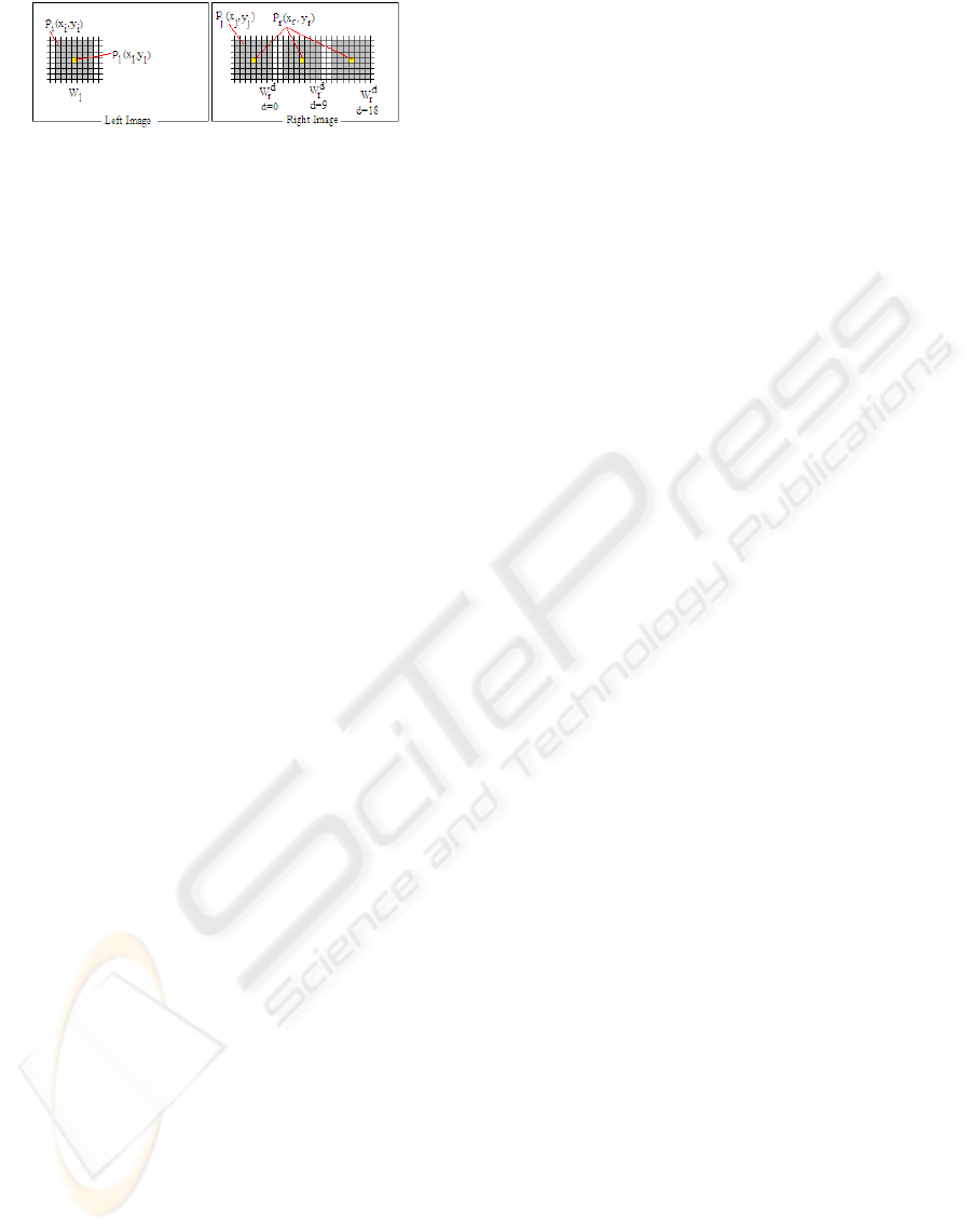
Figure 1: The windows used in DSI Computation.
their high values of intensity, gradient and orientation.
Matching of these points is done using the normalized
correlation (ZNCC) considering the left image to the
right image and vice versa. A valid match is consid-
ered only for those points that yield the best correla-
tion score (Baha and Larabi, 2008). These matched
points will be used in the training of the neural net-
work.
2.1.1 DSI Computation
DSI is an explicit representation of the matching
space introduced by A. Bobik and S. Intille (Bobik
and Intille, 1999). It plays an essential role in the de-
velopment of the overall matching algorithm which
makes use of occlusion constraints.
Assuming that the images pair are rectified, the
disparity computation concerns thus two matched
points which have the same abscise. For each pixel
p
l
(x
l
, y
l
) in the left image, the disparity computation
will concerns all pixels of a window W
l
centered on
p
l
. At each pixel p
i
(x
i
, y
i
) of the W
l
, the matched pixel
p
j
(x
j
, y
j
) will appertains to the window W
d
r
of the
right image centered on p
r
(x
r
, y
r
) (see figure 1). The
position of W
d
r
depends on the disparity d of the pair
(p
l
, p
r
) which varies from zero to d
max
, where d
max
represent the highest disparity value of the stereo-
scopic images. The relations which bind two matched
points p
i
, p
j
of W
l
and W
d
r
are:
x
j
= x
i
+s ∗ d , y
j
= y
i
, where s = ±1 is a sign chosen
so that disparities are always positive.
To determine the disparity of a given pixel
p
l
(x
l
, y
l
), we calculate for assumed disparity d the
score DSI
d
(p
i
) of all p
i
of the windows W
l
. The size
of the window was experimentally chosen to be 7× 7.
In the literature, this score is based only on the pixel
intensities. We introduce in this work two additional
features: the gradient and orientation of pixels. The
DSI
d
(p
i
) score is then computed for a given disparity
d as the sum of squared difference of three attributes
(intensity, gradient magnitude and orientation) as fol-
low:
DSI
d
I
(p
i
) = (I
l
(x
i
, y
i
) − I
r
(x
i
− d, y
i
))
2
(1)
DSI
d
G
(p
i
) = (G
l
(x
i
, y
i
) − G
r
(x
i
− d, y
i
))
2
(2)
DSI
d
O
(p
i
) = (O
l
(x
i
, y
i
) − O
r
(x
i
− d, y
i
))
2
(3)
Where (I
l
, I
r
), (G
l
, G
r
), (O
l
, O
r
) are respectively
the intensities, gradient magnitudes, orientations val-
ues of the pixels on the left and right images.
DSI
d
(p
i
) = DSI
d
I
(p
i
) + DSI
d
G
(p
i
) + DSI
d
O
(p
i
) (4)
To calculate the primary disparity map, This pro-
cess is repeated for each value of the disparity d and
the disparity with the minimal cost DSI
d
(p
l
) among
the various costs of neighboring pixels p
i
of the win-
dow W
l
in the interval [0, dmax ] will be chosen as
the initial disparity of the pixel p
l
and will be noted
d
∗
(p
l
).
As the implementation of this method for DSI
computation is time consuming, we propose in the
next section a neural network architecture in order to
parallelize the calculation of various costs and back
propagation of errors.
2.2 Neural Network Architecture
The proposed neural networks is composed by four-
layer network (see figure 2). The input layer has 147
neurons (3 × 49) of respectively intensities, gradient
magnitudes and orientations of W
l
pixels. The second
layer has the function to compute the scores DSI
d
I
of
intensities, DSI
d
G
of gradient magnitudes and DSI
d
O
of
orientations for each one pixel of the window W
l
. We
obtain then for each value of the disparity d three (7 ×
7) matrices of scores (d = 0..d
max
).
To compute the final DSI
d
, the third layer adds
the three correlation scores for each one pixel of the
window (see equation 4). We obtain d
max
+ 1 ma-
trices of 7 × 7 scores. In the fourth layer, for each
value of d, all scores of the W
l
pixels are added and
constitutes the score SumDSI
d
of the central pixel.
Then, to the central pixel of the window is asso-
ciated a vector of costs (Aggregation cost) AC =
(SumDSI
0
, SumDSI
1
, ..., SumDSI
d
max
). The minimum
cost amount of the d
max
+1 costs is chosen as the best
score and defines the disparity d
∗
of the central pixel
of the window.
The neural correlation network must be trained
with the learning procedure before computing the
minimum of SumDSI
d
values(best score) for each
pixel. To prepare the training data, 150 unmatched
pixels and 50 matched pixels are selected to train of-
fline the network. During training, the differences of
intensities, gradient magnitudes and orientations be-
tween two local windows (one for the left image, the
other for the right) are fed to the network. After the
training, the network should have the ability to differ-
entiate the matched pairs from unmatched ones.
VISAPP 2010 - International Conference on Computer Vision Theory and Applications
356
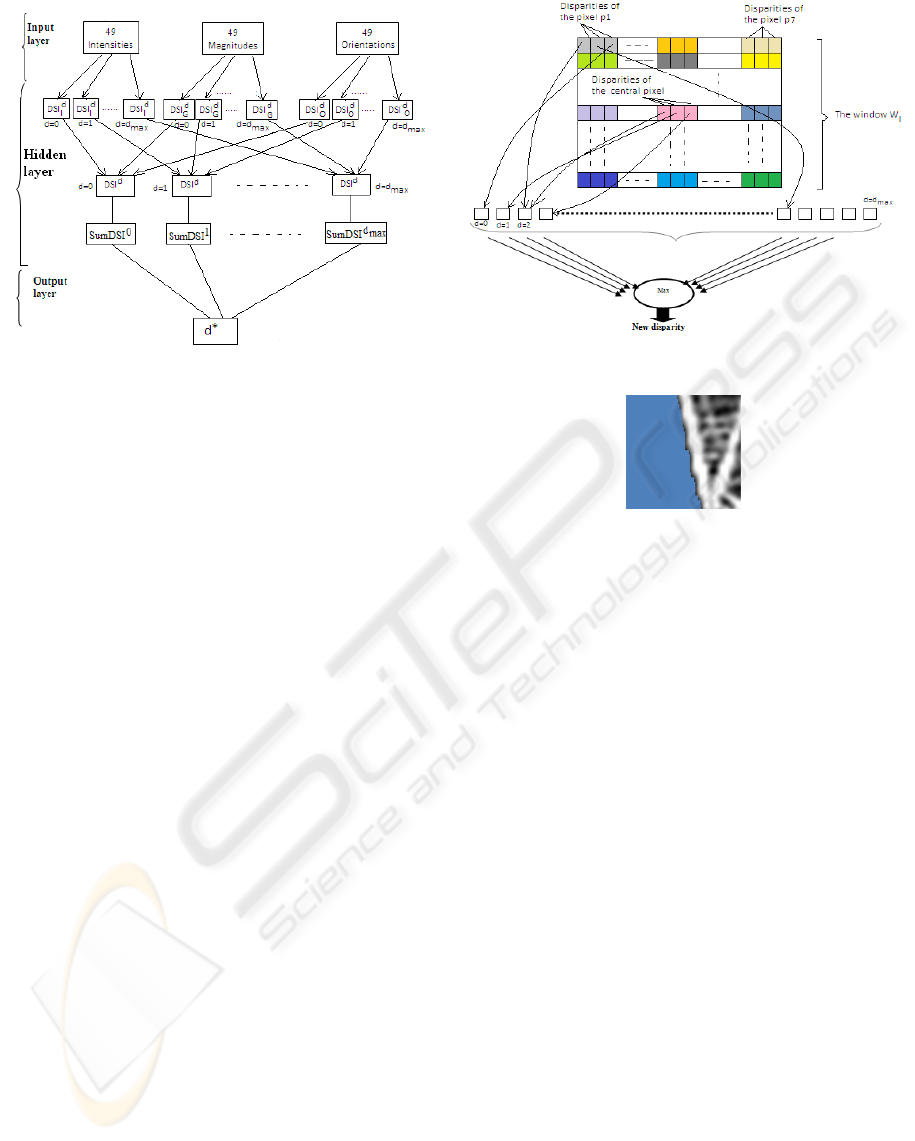
Figure 2: The Neural-DSI network architecture.
3 DISPARITY MAP
REFINEMENT
In this paper we propose the disparity map refinement
by the improvement of Growing Aggregation (GA)
method (Binaghi et al, 2006) and the median filter ap-
plication.
3.1 Improved Growing Aggregation
Unlike conventional techniques that base further steps
of matching algorithm on the minimal aggregated cost
computed, Binaghi bases decisions on the use of all
scores obtained (Binaghi et al, 2006). Instead to se-
lect in the window W
d
l
only one disparity having the
best score, Binaghi propose to select for each pixel n
disparities corresponding to the best scores DSI
d
.
We assume that initial disparities of all pixels of
the left image are computed. For each pixel p
l
of
the left image, we verify in the first if the disparity
is dominant in the window W
l
. If it is the case, this
disparity will be considered as the final disparity and
not necessitates any refinement. Otherwise, we pro-
pose a refinement which consist to select in W
d
l
win-
dow three best scores of SumDSI
d
for each pixel (see
figure 3). We obtain then the best three disparities as-
sociated to the pixel P
l
instead of one disparity. The
proposed process consist to apply a vote in order to
choose the dominant disparity in the associated W
l
us-
ing the three disparities of the central pixel p
l
and its
48 neighboring pixels.
The disadvantage of all known methods published
is that not address the problem of region bound-
aries(see figure 4). For this we propose a second im-
provement of GA method by adding a criterion which
Figure 3: Disparity computing with Improved GA.
Figure 4: Example of inter-region problem.
eliminates from the vote process described above all
pixels of the window W
l
for which the gradient mag-
nitudes have high values relatively to others of the
same window. In this case, only a single disparity
by pixel is considered. Finally, a median filter is used
for smoothing the disparity map.
4 EXPERIMENTS RESULTS
In this section, we describe the experiments con-
ducted to evaluate the performance of the proposed
method. To this purpose, we examine the main algo-
rithms (DSI, Neural network, improved GA and Me-
dian filter). Many applications require not only ac-
curate disparities, but also fast runtime (Nalpantidis
et al, 2008). In our case, we will use the computed
disparity map as input for obstacle detection system.
4.1 Initial Disparity Map Results
To compare the result of initial disparity map with
our method (Neural-DSI), two other approaches were
implemented: The neuronal method and DSI method
as described in (Bobik and Intille, 1999), (Binaghi et
al, 2006). We applied these methods on five images
(Cones, Teddy, Barn1, Sawtooth, Tsukuba) of stan-
dard data sets available on the Middlebury website.
Figures 5 and 6 illustrate the results of initial dis-
TOWARDS REAL-TIME NEURONAL DISPARITY MAP ESTIMATION
357

Figure 5: Initial disparity map obtained with 3 selected
methods.
Figure 6: Processing Time (seconds) of selected algorithms
on the five image pairs.
parity map obtained for 3 selected methods and the
correspondent processing time (second). This time
depends mainly on the image size. The timing tests
were performed on a PC with a microprocessor of 32
bits, 2.5 GHZ. We can clearly see that, the Neural-DSI
method is fastest relatively to DSI and neural meth-
ods.
4.2 Refinement Disparity Map Results
We implemented our method for disparity map refine-
ment(improved GA + median filter) so as the neural
refinement method. The obtained results are illus-
trated by figure 7 and show that our refinement gives
a better map than the neural refinement method.
Figure 8 shows the processing time obtained by
our method (improved GA + median filter) and the
neural refinement method applied on the five image
pairs. Also, the proposed refinement is fastest com-
pared to neural refinement method.
We studied also the influence of window size on
the accuracy of the proposed method. Figure 9 shows
the disparity map obtained after applying our refine-
ment method (improved GA) for the Barn1 image pair
Figure 7: Refinement disparity map obtained with two se-
lected methods.
Figure 8: Processing time (seconds) of the two methods.
for different sizes of the window. More the size of the
window W
l
is great, more the computed map dispar-
ity is good. Nerveless, the computation time is also
very high when the size of W
l
became large. Figure
10 illustrates the variation of time processing for three
methods DSI, Neural and Neural-DSI.
Figure 9: Application of Improved GA method on Barn1
image with different window sizes.
VISAPP 2010 - International Conference on Computer Vision Theory and Applications
358
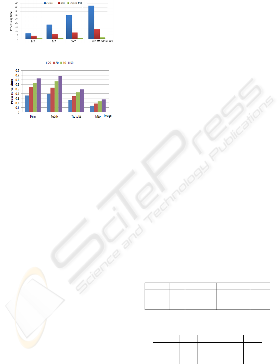
Figure 10: Processing time(s) of the selected methods with
different windows size.
Figure 11: Processing time(s) of disparity map computing
of Neural-DSI with different values of d
max
on four images
pairs with 1x7 window.
Experiments are conducted in order to study the
influence of d
max
values on the performance of the Im-
proved GA method. We used different values of this
parameter for map disparity estimation of four stereo
images pairs with 1x7 window. Figure 11 illustrates
the processing times and show that the Neural-DS I
method is fastest. Indeed, the processing time ob-
tained is less than 0.2seconds.
The results obtained by our algorithm are better
than some methods reported in (Nalpantidis et al,
2008). Indeed the results obtained by (Binaghi et
al, 2004) are satisfactory but not suitable for real-
time applications because the running time needed for
standard image sets is very high. In another method
reported in (Ogale and Aloimonos, 2005), the execu-
tion time varies from 1 to 5 seconds for the standard
image sets . For the window-based method presented
in (Yoon and Kweon, 2006), the running time for the
Tsukuba image pair with 35x35 pixels support win-
dow is about one minute. In the method based on
the Bayesian estimation theory described in (Gutier-
rez and Marroquin, 2004), the results are encouraging
in terms of accuracy but are not suitable for real time
applications, since it takes few minutes to process a
256x255 stereo pair. Another method developed in
(Veksler, 2003), the running times obtained for the
Tsukuba pair is about 6 seconds and 13 seconds for
the Sawtooth pair.
4.3 FPGA Implementation
In order to reduce the computing time, the idea is to
implement certain steps in calculating of the disparity
map on algorithm on a field programmable gate array:
FPGA, the processing time can be further reduced.
Indeed the power of FPGAs has attracted researchers
in computer vision. The use of FPGAs is now the
most convenient and reasonable choice for hardware
development. They are cheap and perform extremely
well (Nalpantidis et al, 2008). Based on the previ-
ous study on the calculation of the disparity map, we
can effectively implement some parts of the methods
that are time consuming using FPGAs circuits of Vir-
tex II. The main objective of this work is the design
of various circuits FPGAs for some algorithm previ-
ously presented using hardware description language
VHDL. For this, we have proposed optimal architec-
tures for:
• The Sobel operator: used to calculate the image
gradient
• Neural-DSI: used for the initial disparity map
• Neural Method: used for the refinement
• The Median Filter: used for the refinement
Due to space limitations in this paper, we present
only the processing time obtained for each compo-
nent. To demonstrate the importance of the use of
FPGA circuits, table 1 illustrates the processing time
obtained for each component in traditional implemen-
tation (Soft) where:
- Pair1, Pair2, pair3 are respectively Barn1(432x381),
Teddy(450x375), Tsukuba(384x288)
- Methods 1, 2, 3, 4 correspond respectively to Gradi-
ent (Sobel), Neural DSI, Neural refinement and Me-
dian Filter.
Table 2 illustrates the processing time obtained for
each component using FPGA implementation. Not
surprisingly the running times obtained with the use
the FPGA are better. All the reasons make FPGA im-
plementation preferable.
Table 1: Processing time (ms) for software implementation.
Method 1 2 3 4
Pair1 147 4.32 × 10
3
31.09 × 10
3
468
Pair2 163 4.81 × 10
3
31.92 × 10
3
470
Pair3 107 3.01 × 10
3
23.06 × 10
3
312.5
Table 2: Processing time (ms) for FPGA implementation.
Method 1 2 3 4
Pair1 2.99 14.991 81.90 3.46
Pair2 3.07 15.369 83.99 3.55
Pair3 2.01 10.072 54.78 2.32
TOWARDS REAL-TIME NEURONAL DISPARITY MAP ESTIMATION
359

5 CONCLUSIONS
The disparity map estimation remains an active area
for research in computer vision. More and more mod-
ern applications demand not only accuracy but real-
time operation as well. In this paper, we presented a
disparity map estimation algorithm based on the neu-
ral network and DSI data structure. The disparity map
computing process is divided on to two main steps.
The first one deals with computing the initial dispar-
ity map using a neuronal method and DSI structure.
The second one presents our contribution to refine the
initial disparity map using improved GA and median
filter so an accurate result can be achieved. Experi-
ments results show that the computation time mainly
depends on the image size, window size and the value
of highest disparity in the image. When we imple-
ment some algorithms on FPGA, the processing time
has decreased considerably.
REFERENCES
Alvarez, L., Deriche, R., Sanchez, J., Weickert, J., (2002).
Dense disparity map estimation respecting image dis-
continuities: a PDE and scalespace based approach..
J. of Visual Commun. Image Represent 13, 3-21.
Baha, N., Larabi, S., (2008). Obstacle Detection from Un-
calibrated Cameras. In Proc of PCI’2008, Greece, pp.
152-157.
Binaghi,, E., Gallo,I., Fornasier, C., Raspanti, M., (2006).
Growing aggregation algorithm for dense two-frame
stereo correspondence. In 1st Int.Conf. on Computer
Vision Theory and Application, 326-332.
Binaghi,, E., Gallo,I., Fornasier, C., Raspanti, M., (2004).
Neural adaptative stereo matching. Pattern Recogni-
tion Letters25,1743-1758.
Bobik,A., Intille,S., (1999). Large occlusion stereo. Intern.
Journal on computer vision 33, 181-200.
Di Stefano, L., Marchionni, M., Mattoccia,S., (2004). A
fast area-based stereo matching algorithm. Image and
vision computing, 22(12), 983-1005.
Goulermas,J., Liatsis,P., (2001). Hybrid symbiotic genetic
optimisation for robust edge-based stereo correspon-
dence. Pattern Recognition. 34, 2477-2496.
Gutierrez, S., Marroquin,J., (2004). Robust approach for
disparity estimation in stereo vision. Image and Vision
Computing, 83-195.
Kumar, S., Chatterji, B., (2002). Stereo matching algo-
rithms based on fuzzy approach. Int. Journal in Pattern
Recognit. Artif. Intell. 16,7, 883-899.
Maas, R.,Haar Romeny, B., Viergever, M., (1999). Area-
based computation of stereo disparity with model
based window size selection. Computer Vision and
Pattern Recognition (CVPR), 106-112.
Miled, W.and Pesquet, J., (2006). Dense Disparity esti-
mation from stereo images. Int. Symposium on Im-
age/Video Communication.
Nalpantidis, L., Sirakoulis, G.,and Gasteratos, A., (2008).
Review of stereo vision algorithms: from Software to
Hardware. International Journal of Optomechatron-
ics, 2:435-462, 2008
Ogale, A., Aloimonos, Y., (2005). Shape and the stereo
Correspondence Problem. Int. Journal of Computer
Vision, 65,3,147-1758.
Scharstein, D., Szeliski,R., (2002). A taxonomy and evalu-
ation of dense two-frame stereo correspondence algo-
rithms. Int. Journal on Computer Vision, 47,7-42.
Veksler, O., (2003). Extracting dense features for visual
correspondence with graph cuts. Proc. Of the IEEE
Computer Society Conference on Computer Vision
and pattern Recognition.
Yoon,K., Kweon,I., (2006). Adaptive Support Weight Ap-
proach for Correspondence Search. IEEE Tran. On
Pattern Analysis and Machine Intelligence, vol. 28.
VISAPP 2010 - International Conference on Computer Vision Theory and Applications
360
