LINEARIZING CONTROL OF YEAST AND BACTERIA FED-BATCH
CULTURES
A Comparison of Adaptive and Robust Strategies
Laurent Dewasme, Alain Vande Wouwer
Service d’Automatique, Universit´e de Mons, 31 Boulevard Dolez, 7000 Mons, Belgium
Daniel Coutinho
Group of Automation and Control Systems, PUCRS, Av. Ipiranga 6681, 90619-900, Porto Alegre, Brazil
Keywords:
Nonlinear robust control, Adaptive control, Fermentation process, Biotechnology.
Abstract:
Linearizing control is a popular approach to control bioprocesses, which has received considerable attention
is the past several years. This control approach is however quite sensitive to modeling uncertainties, thus
requiring some on-line parametric adaptation so as to ensure performance. In this study, this usual adaptive
strategy is compared in terms of implementation and performance to a robust strategy, where the controller
has a fixed parametrization which is determined using a LMI framework so as to ensure robust stability and
performance. Fed-batch cultures of yeast and bacteria are considered as application examples.
1 INTRODUCTION
The culture of host recombinant micro-organisms is
nowadays a very important way of producing bio-
pharmaceuticals. Fed-batch operation is popular in
industrial practice, since it is advantageous from an
operational and control point of view. The off-line
determination of the feeding profile is usually sub-
optimal as some security margin has to be provided
in order to avoid an excess of substrate leading to
the accumulationof inhibitoryby-products(inhibition
of the cell respiratory capacity), namely ethanol for
yeast cultures and acetate for bacteria cultures.
To optimize the culture conditions and to avoid
high concentrations of inhibitory by-products, a
closed-loop solution is required, and a wide diversity
of approaches, e.g., (Pomerleau, 1990; Chen et al.,
1995; Rocha, 2003; Renard and Wouwer, 2008; De-
wasme et al., 2009a; Dewasme et al., 2009b) have
been considered.
In particular, linearizing control (Bastin and
Dochain, 1990) is a very popular approach, which has
been applied successfully in a number of case studies.
However, linearizing control requires the knowledge
of an accurate model, and on-line parametric adap-
tation is usually implemented so as to ensure perfor-
mance. Whereas parametric adaptation is a simple ap-
Substrate
CO
2
Respiro-fermentativeregime
V.P =constant
S= S
crit
Product
Substrate
CO
2
S> S
crit
Respirative regime
S< S
crit
r
o
Substrate
CO
2
Product
CO
2
Product
(r
o
-k
os
r
s
)/k
oa
SubstrateSubstrate
CO
2
Respiro-fermentativeregime
V.P =constant
S= S
crit
Product
Substrate
CO
2
S> S
crit
ProductProduct
Substrate
CO
2
S> S
crit
Respirative regime
S< S
crit
r
o
Substrate
CO
2
Product
CO
2
ProductProduct
(r
o
-k
os
r
s
)/k
oa
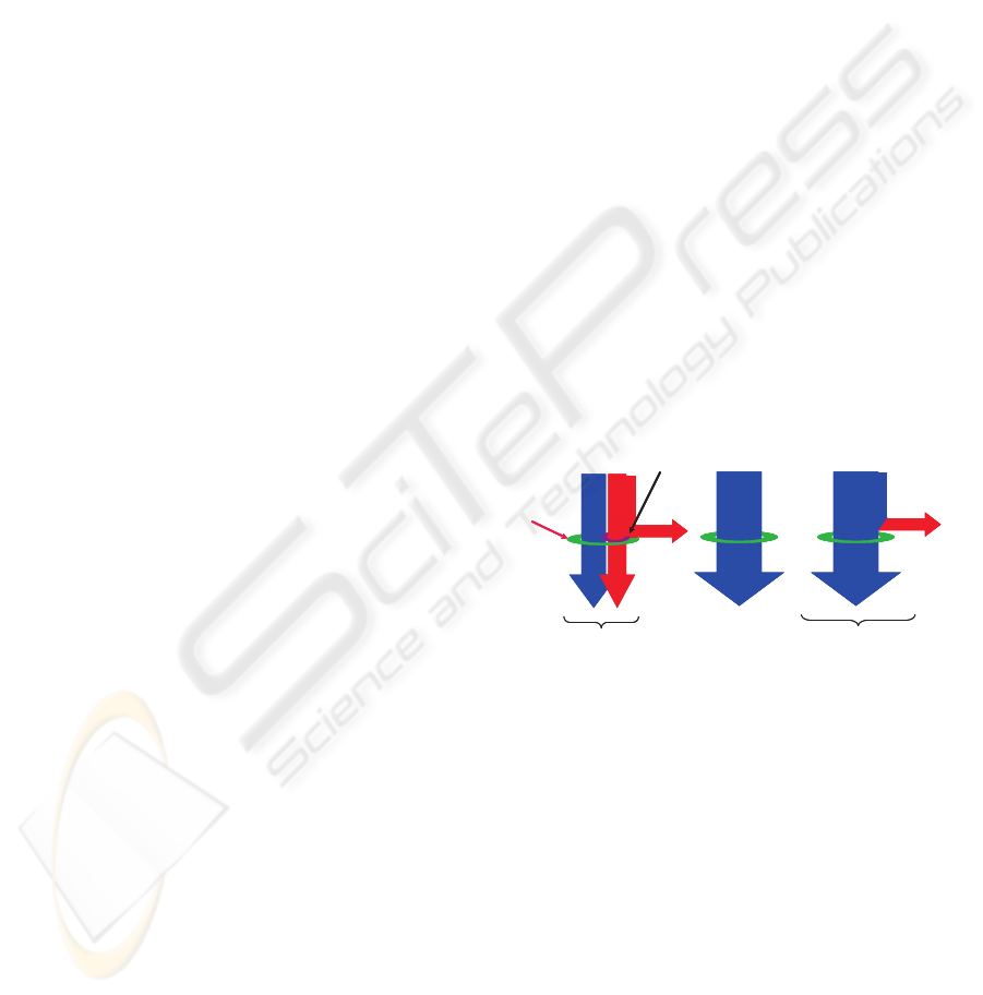
Figure 1: Illustration of Sonnleitner’s bottleneck assump-
tion for cells limited respiratory capacity.
proach, it does not guarantee stability in the presence
of unmodeled dynamics.
In this study, another approach is also considered,
which is based on nonlinear robust control and the
used of Linear Matrix Inequalities (LMIs) to design
the free linear dynamics so as to ensure robust stabil-
ity and performance. A comparison of the adaptive
and robust control approaches is provided in terms
of implementation, and simulation tests shows the re-
spective advantages and limitations of both strategies.
5
Dewasme L., Vande Wouwer A. and Coutinho D. (2010).
LINEARIZING CONTROL OF YEAST AND BACTERIA FED-BATCH CULTURES - A Comparison of Adaptive and Robust Strategies.
In Proceedings of the 7th International Conference on Informatics in Control, Automation and Robotics, pages 5-13
DOI: 10.5220/0002933300050013
Copyright
c
SciTePress

2 MECHANISTIC MODEL
In this study, we consider a generic model that would,
in principle, allow the representation of the culture of
different strains presenting an overflow metabolism
(yeasts, bacteria, animal cells, etc). This model de-
scribes therefore the cell catabolism through the fol-
lowing three main reactions:
Substrate oxidation :
k
S1
S+ k
O1
O
r
1
X
→ k
X1
X+ k
C1
C (1a)
Overflow reaction (typically fermentation) :
k
S2
S+ k
O2
O
r
2
X
→ k
X2
X+ k
P2
P+ k
C2
C (1b)
Metabolite product oxidation :
k
P3
P+ k
O3
O
r
3
X
→ k
X3
X+ k
C3
C (1c)
where X, S, P, O and C are, respectively, the concen-
tration in the culture medium of biomass, substrate
(typically glucose or glycerol), product (i.e. ethanol
or methanol in yeast cultures, acetate in bacteria cul-
tures or lactate in animal cells cultures), dissolved
oxygen and carbon dioxide. k
ξi
(i=1,2,3) are the yield
coefficients and r
1
, r
2
and r
3
are the nonlinear specific
growth rates given by:
r
1
=
min(r
S
,r
S
crit
)
k
S1
(2)
r
2
=
max(0,r
S
− r
S
crit
)
k
S2
(3)
r
3
=
max
0,min
r
P
,
k
os
(r
S
crit
−r
S
)
k
oa
k
P3
(4)
where the kinetic terms associated with the substrate
consumption r
S
, the critical substrate consumption
r
S
crit
(generally dependent on the cells oxidative or
respiratory capacity r
O
) and the product oxidative rate
r
P
are given by:
r
S
= µ
S
S
S+ K
S
(5a)
r
S
crit
=
r
O
k
os
=
µ
O
k
os
O
O+ K
O
Ki
P
Ki
P
+ P
(5b)
r
P
= µ
P
P
P+ K
P
(5c)
These expressions take the classical form of
Monod laws where µ
S
, µ
O
and µ
P
are the maximal val-
ues of specific growth rates, K
S
, K
O
and K
P
are the sat-
uration constants of the corresponding element, and
Ki
P
is the inhibition constant. k
os
and k
oa
represent
the coefficients characterizing respectively the yield
between the oxygen and substrate consumptions, and
the yield between the acetate and oxygen consump-
tions.
This kinetic model is based on Sonnleitner’s bot-
tleneck assumption (Sonnleitner and K¨appeli, 1986)
which was developed for a yeast strain Saccha-
romyces cerevisiae (Figure 1). During a culture, the
cells are likely to change their metabolism because of
their limited respiratory capacity. When the substrate
is in excess (concentration S > S
crit
), the cells produce
a metabolite product P through fermentation, and the
culture is said in respiro-fermentative (RF) regime.
On the other hand, when the substrate becomes lim-
iting (concentration S < S
crit
), the available substrate
(typically glucose), and possibly the metabolite P (as
a substitute carbon source), if present in the culture
medium, are oxidized. The culture is then said in res-
pirative (R) regime.
Component-wise mass balances give the follow-
ing differential equations :
dX
dt
= (k
X1
r
1
+ k
X2
r
2
+ k
X3
r
3
)X − DX (6a)
dS
dt
= −(k
S1
r
1
+ k
S2
r
2
)X + DS
in
− DS (6b)
dP
dt
= (k
P2
r
2
− k
P3
r
3
)X − DP (6c)
dO
dt
= −(k
O1
r
1
+ k
O2
r
2
+ k
O3
r
3
)X − DO+ OTR
(6d)
dC
dt
= (k
C1
r
1
+ k
C2
r
2
+ k
C3
r
3
)X − DC− CTR (6e)
dV
dt
= F
in
(6f)
where S
in
is the substrate concentration in the feed,
F
in
is the inlet feed rate, V is the culture medium vol-
ume and D is the dilution rate (D = F
in
/V). OTR and
CTR represent respectively the oxygen transfer rate
from the gas phase to the liquid phase and the carbon
transfer rate from the liquid phase to the gas phase.
Classical models of OTR and CTR are given by:
OTR = k
L
a(O
sat
− O) (7a)
CTR = k
L
a(P− P
sat
) (7b)
where k
L
a is the volumetric transfer coefficient and,
O
sat
and P
sat
are respectively the dissolved oxygen
and carbon dioxide concentrations at saturation.
3 A SUBOPTIMAL STRATEGY
The maximum of productivity is obtained at the
edge between the respirative and respiro-fermentative
ICINCO 2010 - 7th International Conference on Informatics in Control, Automation and Robotics
6

regimes, where the quantity of by-product is constant
and equal to zero (VP = 0). Unfortunately, evaluating
accurately the volume is a difficult task as it depends
on the inlet and outlet flows including F
in
but also the
added base quantity for pH control and several gas
flow rates. Moreover, maintaining the quantity of by-
productconstant in a fed-batch process means that the
by-product concentration has to decrease while the
volume increases. So, even if the volume is correctly
measured, VP becomes unmeasurable once P reaches
the sensitivity level of the by-productprobe. For those
practical limitations, a sub-optimal strategy is elabo-
rated through the control of the by-product concentra-
tion around a low value P
∗
depending on the sensitiv-
ity of commercially available probes (for instance, a
general order for ethanol probe is 0.1g/l), and requir-
ing only an estimation of the volume by integration of
the feed rate.
The basic principle of the controller is thus to reg-
ulate the by-product at a constant low setpoint, lead-
ing to a self-optimizing control in the sense of (Sko-
gestad, 2004) and ensuring that the culture operates in
the respiro-fermentative regime, close to the biologi-
cal optimum, i.e., close to the edge with the respira-
tive regime.
4 LINEARIZING CONTROL
STRATEGY
The component-wise mass balances of reaction
scheme (1) lead to the following state-space represen-
tation
˙x = Kr(x)X + Ax− ux+ B(u) (8)
where x = [
X S P O C V
]
′
is the state vec-
tor, r(x) = [
r
1
r
2
r
3
]
′
is the vector of reaction
rates, and u = D = F
in
/V is the control input (the di-
lution rate). The matrices K and A, and the vector
function B(·) are given by:
K =
k
X1
k
X2
k
X3
−k
S1
−k
S2
0
0 k
P2
−k
P3
−k
O1
−k
O2
−k
O3
k
C1
k
C2
k
C3
0 0 0
, B(u) =
0
S
in
u
0
k
L
a O
sat
k
L
a P
sat
0
,
(9)
A =
0
3×3
0
3×2
0
3×1
0
2×2
−k
L
a I
2×2
0
2×2
0
1×3
0
1×2
0
,
A feedback linearizing controller is illustrated in
Figure 2. In a first step, this controller is derived as-
suming a perfect process knowledge. The basic idea
Bioreactor
P
X,O
-
+
Controller
u
Process
P*
BioreactorBioreactor
P
X,O
-
+
Controller
u
Process
P*
Figure 2: Linearizing control scheme.
is to derive a nonlinear controller, which allows a lin-
earization of the process behavior ((Chen et al., 1995;
Pomerleau, 1990)).
As the theoretical value of S
crit
is very small (be-
low 0.1 g/l) and assuming a quasi-steady state of S
(i.e. considering that there is no accumulation of glu-
cose when operating the bioreactor in the neighbor-
hood of the optimal operating conditions), the small
quantity of substrate VS is almost instantaneously
consumed by the cells (
d(VS)
dt
≈ 0 and S ≈ 0) and (6b)
becomes:
k
S2
r
2
X = −k
S1
r
1
X + S
in
u (10)
where r
1
and r
2
are nonlinear functions of S, P and O
as given by (2-3).
Replacing r
2
X by (10) in the mass balance equa-
tion for P (6c), we obtain:
˙
P = −
k
P2
k
S1
k
S2
r
1
X − k
P3
r
3
X − u
P−
k
P2
k
S2
S
in
(11)
A first-order linear reference model is imposed:
d(P
∗
− P)
dt
= −λ(P
∗
− P) , λ > 0 (12)
and a constant setpoint is considered so that:
dP
dt
= λ(P
∗
− P) , λ > 0 (13)
Equating (13) and (11), the following control law
is obtained:
F
in
= V
λ(P
∗
− P) + (
k
P2
k
S1
k
S2
r
1
+ k
P3
r
3
)X
k
P2
k
S2
S
in
− P
(14)
where
k
P2
k
S1
k
S2
r
1
and k
P3
r
3
, thekinetic expressions, con-
tain several uncertain parameters.
4.1 A Classical Adaptive Strategy
In (Chen et al., 1995), the parameter uncertainties
are handled using an on-line estimation of the kinetic
term
k
P2
k
S1
k
S2
r
1
+ k
P3
r
3
in the linearizing control law
(14). In this study, the biomass concentration X is
supposed to be measured using a probe (for instance
LINEARIZING CONTROL OF YEAST AND BACTERIA FED-BATCH CULTURES - A Comparison of Adaptive and
Robust Strategies
7

a optical density probe or a conductance probe, which
are nowadays widely available), whereas in (Chen
et al., 1995), an asymptotic observer is used to es-
timate this component concentration. The following
adaptive scheme is therefore a simplified version of
the original algorithm.
F
in
= V
λ(P
∗
− P) +
ˆ
θX
k
P2
k
S2
S
in
− P
(15)
A direct adaptive scheme as described in (Bastin
and Dochain, 1990) is used. Consider the following
Lyapunov function candidate:
V(t) =
1
2
˜
P
2
+
˜
θ
2
γ
(16)
where
˜
P = P
∗
−P,
˜
θ = θ−
ˆ
θ and γ is a strictly positive
scalar. The specific growth rates r
1
and r
3
(and, of
course, the pseudo-stoichiometric coefficient k
4
) are
assumed to be constant so that θ variations are negli-
gible (
dθ
dt
= 0).
Using the Lyapunov stability theory, the time
derivative of the Lyapunov candidate function should
be negative for the closed-loop system to be stable:
dV
dt
=
d
˜
P
dt
˜
P+
˜
θ
d
˜
θ
dt
1
γ
(17)
Considering (13) and a possible parameter mis-
match (
ˆ
θ 6= θ):
d
˜
P
dt
= −λ
˜
P−
˜
θX (18)
so that (17) becomes:
dV
dt
= −λ
˜
P
2
−
˜
P
˜
θX −
˜
θ
d
ˆ
θ
dt
1
γ
(19)
Choosing the following θ adaptive law cancels the
second and the third terms:
d
ˆ
θ
dt
= γX
˜
P (20)
4.2 A Robust Strategy
Structural and parametric uncertainties can be lumped
into a global parametric error:
δ =
¯
θ− θ (21)
where δ is a nonlinear function of (S,P,O) represent-
ing possible inexact cancellations of nonlinear terms
due to model uncertainties and
¯
θ represents the hypo-
thetical exact unknown value. Rewriting the kinetic
term in (15) using the newexpression taken from (21),
we obtain:
u = F
in
= V
λ(P
∗
− P) +
¯
θX − δX
k
P2
k
S2
S
in
− P
(22)
which corresponds to the perturbed reference system:
˙
P = λ(P
∗
− P) − δX (23)
Borrowing the ideas of the Quasi-LPV approach
(Leith and Leithead, 2000), we bound the time-
varying parameter δ which is supposed to belong to
a known set ∆ := {δ : δ ≤ δ ≤ δ} with δ and δ respec-
tively representing the minimal and maximal admis-
sible uncertainties.
The parameter λ is designed to ensure some ro-
bustness and tracking performance to the overall
closed-loop system, which is modeled as follows:
M :
˙
P = −λz− δX
z = P
∗
− P
(24)
where z = P
∗
− P is the performance output.
Let w = [
P
∗
X
]
′
⊂ L
2,[0,T]
be the disturbance
input to the system M , a(λ, δ) =
λ −δ
and
c =
1 0
. The closed-loop system (24) can be
rewritten:
M :
˙
P = −λP+ a(λ, δ)w
z = − P + c w , δ ∈ ∆
(25)
Consider the finite horizon (for instance, between
the instant 0 and the time T) L
2
-gain of system M
(M. Green and D.J.N. Limebeer, 1994), representing
the worst-case of the ratio of kzk
2,[0,T]
(i.e., the finite
horizon 2-norm of the tracking error) and kwk
2,[0,T]
(i.e., the finite horizon 2-norm of the disturbance in-
put), which is defined as:
kM
wz
k
∞,[0,T]
= sup
δ∈∆,06=w⊂L
2,[0,T]
kzk
2,[0,T]
kwk
2,[0,T]
(26)
Thus, the parameter λ is designed based on the H
∞
control theory (M. Green and D.J.N. Limebeer, 1994;
Skogestad and Postlethwaite, 2001). Let α > 0 be an
upper limiting of kM
wz
k
∞,[0,T]
. Thus, the problem is
to find α such that:
min
λ,δ∈∆
α : kM
wz
k
∞,[0,T]
≤ α (27)
while ensuring the robust stability of system (25).
This optimization problem can be written in terms
of linear matrix inequalities (LMIs) and solved us-
ing readily available toolboxes, e.g., SeDuMi (Sturm
et al., 2006) can be applied to solve the prob-
lem. These constraints can be easily obtained via a
quadratic Lyapunov function (S.Boyd, L.El-Ghaoui,
E.Feron and V.Balakrishnan, 1994)
V(P) = P
′
QP = QP
2
(28)
where Q is a strictly positive symmetric matrix (i.e.,
Q = Q
′
≻ 0) and ”
′
” corresponds to the transposition
matrix operation.
ICINCO 2010 - 7th International Conference on Informatics in Control, Automation and Robotics
8

The minimization in (27) is then equivalent to:
min α : V(P) ≻ 0 ,
˙
V(P) +
1
α
z
′
z− αw
′
w ≺ 0 (29)
where, using (25) and (28), the time derivative of
V(P) is given by:
˙
V(P) =
˙
P
′
QP+ P
′
Q
˙
P
= (−λP+ aw)
′
QP+ P
′
Q(−λP+ aw)
= −λP
′
QP+ (aw)
′
QP− λP
′
QP+ P
′
Qaw
= −2λP
′
QP+ a
′
w
′
QP+ P
′
Qaw (30)
Using (30) in (29), the following expression is ob-
tained:
P
w
′
−2m Qa
a
′
Q −αI
n
w
P
w
−
1
α
zz
′
≺ 0 (31)
where m = λQ and I
n
w
is the unity matrix of dimen-
sion n
w
× n
w
and n
w
is the dimension of w.
Now, consider the following lemma (Schur Com-
plement):
Lemma 1. The following matrix inequalities are
equivalent
(i) T > 0,R − ST
−1
S
′
≻ 0
(ii) R > 0, T − S
′
R
−1
S ≻ 0
(iii)
R S
S
′
T
≻ 0
Hence, using the expression of z,a and c in (25)
and Lemma 1, the optimization problem in (27) can
be written as follows:
min
Q,m
α : α > 0 , Q = Q
′
> 0 and
−2m m −δQ −1
m −α 0 1
−δQ 0 −α 0
−1 1 0 −α
≺ 0 (32)
If there exists a feasible solution to the above op-
timization problem for all δ evaluated at the vertices
of ∆, then (27) is satisfied and λ = mQ
−1
.
Remark 1. Quadratic Lyapunov functions may be
conservative for assessing the stability of parameter-
dependent systems (G. Chesi and Vicino, 2004).
However, a parameter-independent Lyapunov func-
tion is considered in this study for two main reasons:
1. λ is parametrized with the Lyapunov matrix Q
so as to obtain a convex design condition. A
parameter-independent matrix Q therefore results
in a parameter-independent control law;
2. the variation of δ is a priori unknown.
Remark 2. This method is likely to be conservative,
as the parameter δ has to bound the nonlinearities
of the inexactly cancelled terms. Less conservative
results can be obtained by considering the approach
of (D.F. Coutinho, M. Fu, A. Trofino and P. Dan`es,
2008) to deal with the nonlinearities at the cost of a
larger computational effort.
5 NUMERICAL RESULTS
In this section, for comparing the adaptive and ro-
bust linearizing control strategies, several numeri-
cal simulations considering small-scale bacteria and
yeast cultures (respectively in 5 and 20 [l] bioreac-
tors) are performed. The first simulation set is dedi-
cated to yeast cultures with initial and operating con-
ditions: X
0
= 0.4g/l, S
0
= 0.5g/l, E
0
= 0.8g/l, O
0
=
O
sat
= 0.035g/l, C
0
= C
sat
= 1.286g/l, V
0
= 6.8l,
S
in
= 350g/l. The second simulation set is dedicated
to bacteria cultures with initial and operating condi-
tions: X
0
= 0.4g/l, S
0
= 0.05g/l, A
0
= 0.8g/l, O
0
=
O
sat
= 0.035g/l, C
0
= C
sat
= 1.286g/l, V
0
= 3.5l,
S
in
= 250g/l
The values of all model parameters are listed in
Tables 1, 2, 3 and 4. Note that, for yeast cultures,
coefficients k
os
and k
oa
are simply replaced by k
O1
and k
03
while k
O2
= 0, in accordance with the model
of (Sonnleitner and K¨appeli, 1986). For the bacte-
ria model, parameters values are taken from (Rocha,
2003) and slightly modified to adapt the yield coeffi-
cient normalization to the proposed reaction scheme
(1) and kinetic model (with a slight difference in the
formulation of r
3
).
The state variables are assumed available (i.e.,
measured) online for feedback. The adaptive and ro-
bust linearizing feedback controllers proposed in sec-
tion 4 aim at tracking the byproduct set-point (E
∗
and
A
∗
= 1 g/l) which is chosen sufficiently low so as to
stay in the neighborhood of the optimal trajectory but
also sufficiently high to avoid probe sensitivity limi-
tations. In this setup, a noisy byproduct measurement
is considered.
To design the parameter λ in (23) via the optimiza-
tion problem (27), the parameters K
S
, K
P
, K
O
, K
i
P
and µ
S
, µ
O
are assumed to be respectively varying of
±100% and ±15% from their nominal values. Simu-
lating the operating conditions of the control strategy
in (22), we may infer that δ = −δ = 0.5/3600 s
−1
for
yeast cultures and δ = −δ = 0.1/3600 s
−1
for bac-
teria cultures. In light of (25) and (27), these con-
straints yield for yeasts and bacteria, respectively to
λ = 0.0056 and λ = 0.0046.
Concerning the adaptive control law, λ = 1 and
LINEARIZING CONTROL OF YEAST AND BACTERIA FED-BATCH CULTURES - A Comparison of Adaptive and
Robust Strategies
9
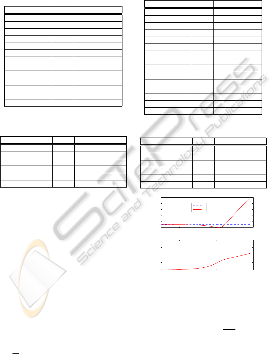
Table 1: Yield coefficients values of Sonnleitner and
K¨appeli for S. cerevisiae model (Sonnleitner and K¨appeli,
1986)
Yield coefficients Values Units
k
X1
0,49 g of X/g of S
k
X2
0,05 g of X/g of S
k
X3
0,72 g of X/g of E
k
S1
1
k
S2
1
k
P2
0,48 g of E/g of S
k
P3
1
k
O1
0,3968 g o f O
2
/g of S
k
O2
0 g of O
2
/g of S
k
O3
1,104 g of O
2
/g of E
k
C1
0,5897 g of CO
2
/g of S
k
C2
0,4621 g of CO
2
/g of S
k
C3
0,6249 g of CO
2
/g of E
Table 2: Kinetic coefficients values of Sonnleitner and
K¨appeli for the S. cerevisiae model (Sonnleitner and
K¨appeli, 1986)
Kinetic coefficients Values Units
µ
O
0,256 g of O
2
/g of X /h
µ
S
3,5 g of S/g of X /h
K
O
0,0001 g of O
2
/l
K
S
0,1 g of S/l
K
E
0,1 g of E/l
Ki
E
10 g of E/l
γ = 0.05 for yeast cultures while λ = 2 and γ = 0.25
for bacteria cultures. Note also that the sampling pe-
riod is chosen equal to 0.1 h.
Before discussing the results of the proposed
methods, it is interesting to observe the performance
of a plain linearizing controller, i.e. without adapta-
tion or robustification, applied to the yeast process in
the presence of modeling errors. For instance, con-
sider the situation where the user selects a relatively
high gain λ = 1, and
ˆ
θ is fixed to k
P2
/2. Figure 3 illus-
trates the consequences of such choices. Even if the
controller behaves correctly during the first hours, the
divergence of the ethanol signal during the last hours
will impact the quality of the culture.
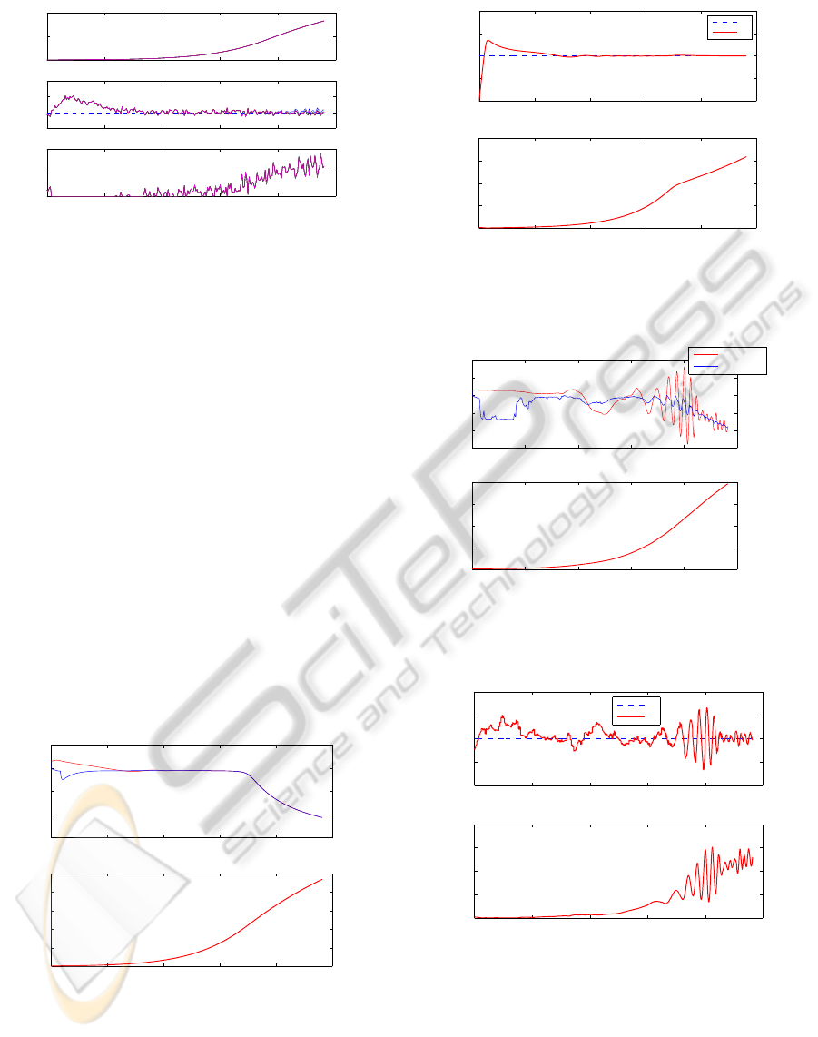
Figure 4 shows now the closed-loop response of
biomass X, ethanol E concentrations, and the inlet
feed rate F
in
, for five different values of the kinetic
parameters (which were randomly chosen) in yeast
cultures under a robust control strategy. In all sim-
ulation runs, a white noise is added to the ethanol
concentration measurement with a standard deviation
of ±0.1 [g/l] and the culture is considered as always
evolving in the optimal operating conditions in which
r
1
=
r
O
k
O1
and r
3
= 0 so that the hypothetical parameter
Table 3: Yield coefficients values of Rocha’s E.coli model
(Rocha, 2003)
Yield coefficients Values Units
k
X1
1
k
X2
1
k
X3
1
k
S1
0,316 g of S/g of X
k
S2
0,04 g of S/g of X
k
P2
0,157 g of A/g of X
k
P3
0,432 g of A/g of X
k
O1
0,339 g of O
2
/g of X
k
O2
0,471 g of O
2
/g of X
k
O3
0,955 g of O
2
/g of X
k
C1
0,405 g of CO
2
/g of X
k
C2
0,754 g of CO
2
/g of X
k
C3
1,03 g of CO
2
/g of X
k
os
2,02 g of O
2
/g of X
k
oa
1,996 g of O
2
/g of X
Table 4: Kinetic coefficients values of Rocha’s E.coli
model (Rocha, 2003)
Kinetic coefficients Values Units
µ
O
0,7218 g of O
2
/g of X /h
µ
S
1,832 g of S/g of X /h
K
O
0,0001 g of O
2
/l
K
S
0,1428 g of S/l
K
A
0,5236 g of A/l
Ki
A
6,952 g of A/l
0 5 10 15 20 25
0
2
4
6
8
10
E [g/l]
E*
E
0 5 10 15 20 25
0
1
2
3
4
x 10
−4
F
in
[l/s]
Time [h]
Figure 3: Yeast cultures – ethanol concentration and feed
rate when the controller is designed using a plain linearizing
control approach (no adaptation and no robustification) in
the presence of modeling errors.
¯
θ in (22) is taken as
¯
θ =
˜
k
P2
k
S1
k
S2
r
1
+
˜
k
P3
r
3
≈
k
P2
k
S1
k
S2
r
O
k
O1
(33)
Figure 4 shows that during the start-up phase, F
in
saturates to 0, leading to an ethanol overshoot (see
ICINCO 2010 - 7th International Conference on Informatics in Control, Automation and Robotics
10
0 5 10 15 20 25
0
50
100
X [g/l]
0 5 10 15 20 25
0
1
2
3
E [g/l]
0 5 10 15 20 25
0
2
4
x 10
−4
Time [h]
F
in
[l/s]
Figure 4: Yeast cultures – biomass and ethanol concentra-
tions, and feed rate – robust control strategy – results of 5
runs with random parameter variations and a noise standard
deviation of ±0.1 [g/l].
Figure 4). The different curves are more or less indis-
tinguishable (the same noise signal is applied during
the 5 runs) except in the last hours where the conse-
quences of model errors appear. Nevertheless, these
results are very satisfactory as model errors have a
negligible influence.
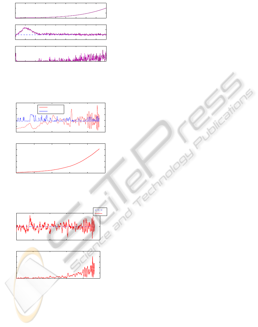
Figures 5 and 6 show the results of a simulation
performed with the same initial and operating con-
ditions with the adaptive strategy, in the ideal case
where there is no measurement noise, whereas Fig-
ures 7 and 8 correspond to a noise standard devia-
tion of ±0.05 [g/l] added to the ethanol concentra-
tion measurements. Due to sensitivity problems of
the adaptive law, higher noise levels usually lead to
computational failures. When the parameter adapta-
tion performs well, the productivity of the adaptive
and robust strategies is more or less the same, i.e., a
biomass concentration of approximately 80 g/l is ob-
tained within 24 hours.
0 5 10 15 20 25
2
4
6
8
10
x 10
−5
θ adaptation
θ [s
−1
]
0 5 10 15 20 25
0
20
40
60
80
100
X [g/l]
Time [h]
Figure 5: Yeast cultures – θ adaptation and biomass concen-
tration – adaptive control strategy – no measurement noise.
Figure 9 shows the closed-loop response of
biomass X, acetate A concentrations, and inlet feed
rate F
in
, for five different values of the kinetic pa-
rameters which are randomly chosen, in the bacteria
0 5 10 15 20 25
0.8
0.9
1
1.1
1.2
E [g/l]
E*
E
0 5 10 15 20 25
0
1
2
3
4
x 10
−4
F
in
[l/s]
Time [h]
Figure 6: Yeast cultures – ethanol concentration and feed
flow rate – adaptive control strategy – no measurement
noise.
0 5 10 15 20 25
2
4
6
8
10
12
x 10
−5
θ adaptation
θ [s
−1
]
0 5 10 15 20 25
0
20
40
60
80
X [g/l]
Time [h]
Estimated θ
Real θ
Figure 7: Yeast cultures – θ adaptation and biomass concen-
tration – adaptive control strategy – noise standard deviation
of ±0.05 [g/l].
0 5 10 15 20 25
0
0.5
1
1.5
2
E [g/l]
E*
E
0 5 10 15 20 25
0
1
2
3
4
x 10
−4
F
in
[l/s]
Time [h]
Figure 8: Yeast cultures – ethanol concentration and feed
flow rate – adaptive control strategy – noise standard devia-
tion of ±0.05 [g/l].
cultures under a robust control strategy. Figures 10
and 11 show similar simulation runs with the adap-
tive strategy. The same comments concerning the
noise sensitivity apply.
Note that the productivity is lower in the bacteria
LINEARIZING CONTROL OF YEAST AND BACTERIA FED-BATCH CULTURES - A Comparison of Adaptive and
Robust Strategies
11
0 5 10 15 20 25 30 35 40 45
0
10
20
30
X [g/l]
0 5 10 15 20 25 30 35 40 45
0
1
2
3
A [g/l]
0 5 10 15 20 25 30 35 40 45
0
0.5
1
x 10
−4
Time [h]
F
in
[l/s]
Figure 9: Bacteria cultures – biomass and acetate concen-
trations, and feed rate – robust control strategy – results of 5
runs with random parameter variations and a noise standard
deviation of ±0.1 [g/l].
0 10 20 30 40 50
0
0.2
0.4
0.6
0.8
1
x 10
−4
θ adaptation
θ [s
−1
]
0 10 20 30 40 50
0
5
10
15
20
25
X [g/l]
Time [h]
Estimated θ
θ
Figure 10: Bacteria cultures – θ adaptation and biomass
concentration – adaptive control strategy – noise standard
deviation of ±0.05 [g/l].
0 10 20 30 40 50
0.5
1
1.5
A [g/l]
A*
A
0 10 20 30 40 50
0
0.2
0.4
0.6
0.8
1
x 10
−4
F
in
[l/s]
Time [h]
Figure 11: Bacteria cultures – acetate concentration and
feed flow rate – adaptive control strategy – noise standard
deviation of ±0.05 [g/l].
cultures (for biological and operating reasons, bacte-
ria strains lead to reaction rates and, therefore, growth
rates that are smaller than yeast reaction rates). How-
ever, from a control point of view, results are satisfac-
tory in both cases.
6 CONCLUSIONS
Linearizing control is a powerful approach to the con-
trol of fed-batch bioprocesses. In most applications
reported in the literature, on-line parameter adapta-
tion is proposed in order to ensure the control per-
formance despite modeling uncertainties. On-line pa-
rameter adaptation is however sensitive to measure-
ment noise, and requires some kind of tuning. On
the other hand, robust control provides an easy design
procedure, based on well established computational
procedures using the LMI formalism. Large paramet-
ric and structural uncertainties, as well as measure-
ment noise levels can be dealt with.
ACKNOWLEDGEMENTS
This paper presents research results of the Belgian
Network DYSCO (Dynamical Systems, Control, and
Optimization), funded by the Interuniversity Attrac-
tion Poles Program, initiated by the Belgian State,
Science Policy Office. The scientific responsibility
rests with its authors.
REFERENCES
Bastin, G. and Dochain, D. (1990). On-Line Estimation and
Adaptive Control of Bioreactors, volume 1 of Process
Measurement and Control. Elsevier, Amsterdam.
Chen, L., Bastin, G., and van V. Breusegem (1995). A case
study of adaptive nonlinear regulation of fed-batch bi-
ological reactors. Automatica, 31(1):55–65.
Dewasme, L., Richelle, A., Dehottay, P., Georges, P., Remy,
M., Bogaerts, P., and Wouwer, A. V. (2009a). Lin-
ear robust control of s. cerevisiae fed-batch cultures
at different scales. In press, Biochemical Engineering
Journal.
Dewasme, L., Wouwer, A. V., Srinivasan, B., and Per-
rier, M. (2009b). Adaptive extremum-seeking con-
trol of fed-batch cultures of micro-organisms exhibit-
ing overflow metabolism. In Inproceedings of the AD-
CHEM conference in Istanbul (Turkey).
D.F. Coutinho, M. Fu, A. Trofino and P. Dan`es (2008). L2-
gain analysis and control of uncertain nonlinear sys-
tems with bounded disturbance inputs. Int’l J. Robust
Nonlinear Contr., 18(1):88–110.
G. Chesi, A. Garulli, A. T. and Vicino, A. (2004). Robust
analysis of LFR systems through homogeneous poly-
nomial Lyapunov functions. 49, (7):1211–1215.
Leith, D. and Leithead, W. (2000). Survey of gain-
scheduling analysis and design. International Journal
of Control, 73:1001–1025.
M. Green and D.J.N. Limebeer (1994). Linear Robust Con-
trol. Prentice Hall.
ICINCO 2010 - 7th International Conference on Informatics in Control, Automation and Robotics
12

Pomerleau, Y. (1990). Mod´elisation et commande d’un
proc´ed´e fed-batch de culture des levures pain. PhD
thesis, D´epartement de g´enie chimique. Universit´e de
Montr´eal.
Renard, F. and Wouwer, A. V. (2008). Robust adaptive con-
trol of yeast fed-batch cultures. Comp. and Chem.
Eng., 32:1238–1248.
Rocha, I. (2003). Model-based strategies for computer-
aided operation of recombinant E. coli fermentation.
PhD thesis, Universidade do Minho.
S.Boyd, L.El-Ghaoui, E.Feron and V.Balakrishnan (1994).
Linear Matrix Inequalities in System and Control The-
ory. SIAM.
Skogestad, S. (2004). Control structure design for complete
chemical plants. Computers and Chemical Engineer-
ing, 28(1-2):219–234.
Skogestad, S. and Postlethwaite, I. (2001). Multivariable
Feedback Control - Analysis and Design. John Wiley
& Sons, New York, NJ.
Sonnleitner, B. and K¨appeli, O. (1986). Growth of
Saccharomyces cerevisiae is controlled by its limited
respiratory capacity : Formulation and verification of
a hypothesis. Biotechnol. Bioeng., 28:927–937.
Sturm, J. F., Romanko, O., and Plik, I. (2006). SeDuMi,
version 1.1R3. Online – http://sedumi.mcmaster.ca/.
LINEARIZING CONTROL OF YEAST AND BACTERIA FED-BATCH CULTURES - A Comparison of Adaptive and
Robust Strategies
13
