
DISTRIBUTED KALMAN FILTER-BASED TARGET TRACKING
IN WIRELESS SENSOR NETWORKS
Phuong Pham and Sesh Commuri
School of Electrical and Computer Engineering, The University of Oklahoma
110 W. Boyd St., Devon Energy Hall 150, Norman, Oklahoma 73019-1102, U.S.A.
Keywords: Distributed Kalman Filter, Wireless Sensor Networks, and Target Tracking.
Abstract: The tracking of mobile targets using Distributed Kalman Filters in a Wireless Sensor Network (WSN) is
addressed in this paper. In contrast to the Kalman Filter implementations reported in the literature, our
approach has the Kalman Filter running on only one network node at any given time. The knowledge
learned by this node, i.e. the system state and the covariance matrix, is passed on to the subsequent node
running the filter. Since a finite subset of the sensor nodes is active at any given time, target tracking can be
accomplished using lower power compared to centralized implementations of the Kalman Filter. Numerical
simulations demonstrate that the proposed algorithm is robust to measurement noise and changes in the
velocity of the target. The results in this paper show that the proposed technique for target tracking will
result in significant savings in power consumption and will extend the useful life of the WSN.
1 INTRODUCTION
Surveillance of remote inaccessible areas and the
detection and tracking of intruders are some of the
important applications of Wireless Sensor Networks
(WSNs). Research in WSNs has addressed several
important issues in optimal deployment, coverage,
routing, and energy efficiency of the WSNs
(Akyildiz, Su, Sankarasubramaniam, and Cayirci,
2002; Al-Karaki and Kamal, 2004; Cardei, Thai, Li,
and Wu, 2005; Chiang, Wu, Liu, and Gerla, 1997;
Watfa and Commuri, 2006a, 2006b) Diffusion and
directed diffusion approaches have been proposed to
address coverage, routing, discovering, and sensing
fusion issues in WSNs (Intanagonwiwat, Govindan,
and Estrin, 2000). The application of WSNs in
surveillance and monitoring of target areas have also
been widely researched (Chen, Gonzalez, and
Leung, 2007). While the results presented in these
papers are encouraging, their applicability in low
cost WSNs with large measurement noise and faulty
measurements is fraught with problems. In recent
years, Kalman Filters have been proposed to address
the uncertainty and the noise in the measurements
(Rao and Durrant-Whyte, 1991; Olfati-Saber, 2007;
Alriksson and Rantzer, 2007; Olfati-Saber and
Shamma, 2005; Cattivelli, Lopes, and Sayed, 2008;
Uhlmann, 1996; Kim, West, Scholte, and
Narayanan, 2008; Mutambara, 1998; Hashemipour,
Roy, and Laub, 1998). Both centralized and
distributed implementation of the Kalman Filter was
proposed to make their use suitable to WSN
applications. However, these techniques are still
power intensive and require significant amounts of
onboard power for communication and computation.
Two classes of Kalman filtering approaches have
been implemented in WSNs. The first approach is
centralized Kalman Filters (Rao, et al., 1991) where
every sensor node takes measurements and
communicates with the other nodes while
simultaneously performing its own version of
Kalman Filter. In this approach, the sensor nodes’
power will be depleted quickly because of excessive
measurements and inter-node communication.
Moreover, it is sometimes impractical for a sensor
node to communicate with all the other nodes due to
limitation of communication ranges. The second
method is distributed Kalman Filters (Olfati-Saber,
2007; Olfati-Saber, et al., 2005; Cattivelli, et al.,
2008) where every neighbor node runs its own
version of the Kalman Filter and shares the
information with all other neighbors to reach the
consensus of the system. The approaches above are
distributed in processing. The number of neighbor
nodes determines how expensive the algorithms are
54
Pham P. and Commuri S. (2010).
DISTRIBUTED KALMAN FILTER-BASED TARGET TRACKING IN WIRELESS SENSOR NETWORKS.
In Proceedings of the 7th International Conference on Informatics in Control, Automation and Robotics, pages 54-61
DOI: 10.5220/0002952900540061
Copyright
c
SciTePress

in terms of power consumption and communication
complexity. Consequently, these approaches are not
efficient because they require extensive inter-
communication among neighbor nodes. In
comparison with the distributed version of Kalman
Filter in literature (Rao, et al., 1991; Olfati-Saber,
2007; Alriksson, et al., 2007; Olfati-Saber, et al.,
2005; Cattivelli, et al., 2008; Hashemipour, et al.,
1998), our version of the distributed Kalman Filter
simplifies computational burden and reduces inter-
node communication. Thus, the total power
consumption in the entire sensor network is lower
than that reported elsewhere in the literature.
Our approach is different from the above work in
the sense that the Kalman Filter is implemented in a
distributed fashion across the WSNs. At a given
instant, only one master node runs the Kalman Filter
using the measurement inputs from its neighbors and
shares the estimated knowledge with the subsequent
master node. The neighbors within a certain distance
from the target measure the distance to the target,
and transmit measurements to the master node. On
one hand, the procedure significantly reduces the
communication costs among the neighbor nodes in
comparison with the algorithms proposed in (Rao, et
al., 1991; Olfati-Saber, 2007; Alriksson, et al., 2007;
Olfati-Saber, et al., 2005; Cattivelli, et al., 2008;
Hashemipour, et al., 1998). On the other hand, since
the master node alone executes the Kalman Filter
and the neighbor nodes only perform measurement
functions, the complexity of the WSN is greatly
reduced.
Another contribution of this paper is that the
master node determines the direction and velocity of
the intruder and wakes up appropriate sensor nodes
in the direction of the target travel. As the target
moves into the sensing range of a sensor node, it is
already activated and is ready to take measurements.
Whereas the other nodes that are far away from the
target are automatically turned off to save energy.
The master node also decides to wake up sufficient
nodes to take measurements. By knowing the
maximum target’s velocity, the boundary nodes of
the sensor field are activated in round robin fashion
discussed in (Watfa, et al., 2006b) to save energy.
Unlike other approaches mentioned above, we
do not make an assumption about the linear
movement of the target. In this paper, the distributed
Kalman Filter is proposed to estimate the position of
the target. This approach is validated through
simulation examples and the results are compared
with those represented in literature. We show the
main contribution, the approach, validations, and
comparison between our method and the previous
work on distributed Kalman filtering. The algorithm
was also able to track the target with random
directions with acceptable estimated results. The
estimation results showed that the model is robust to
measurement noise and the change in velocity. The
estimated knowledge of the Kalman Filter including
system state and covariance matrix is passed directly
to the subsequent master node where the Kalman
Filter is run. Consequently, the performance of the
distributed Kalman Filter is as good as that of the
centralized Kalman Filter.
The rest of the paper is organized as follows:
Section 2 discusses the algorithm in details. In
section 3, we show the numerical simulation.
Section 4 and 5 are discussion and conclusion.
2 ALGORITHM
2.1 Problems and Assumptions
A sensor field is densely deployed with sensor
nodes. It is assumed that each node has
omnidirectional sensing capability to measure the
distance between the target and itself. Moreover,
every node knows its coordinates in the sensor field,
and all nodes are stationary. Initially, all the nodes
except those at the boundary of the monitored area
are assumed to be in sleep mode. Assuming that
there is an intruder entering the sensor field with an
unknown nonlinear trajectory and a known
maximum velocity, the problem is to track the
position of the intruder accurately. When a target
moves in the sensor field, the nodes close to the
target will automatically activate and sense the
target.
All sensing nodes are within one communication
hop from the master node. The trilateration
algorithm requires that every point in the field is
covered by at least three sensor nodes.
A node can be either the master node or a
measurement node. Nodes take measurements and
sends data to the master node if they are actively in
the sensing region. Concurrently, the master node
collects data from its neighbors, running estimation
algorithms and broadcasting the information of the
target to its neighbors, including the target’s current
coordinates and direction. Depending on the
information from the master node, the neighbor
nodes around the target automatically turn off when
they are not in the region of activation R around
which is defined as the following .
The target, represented by symbol shown in
Figure 1, is moving in horizontal direction. The
DISTRIBUTED KALMAN FILTER-BASED TARGET TRACKING IN WIRELESS SENSOR NETWORKS
55
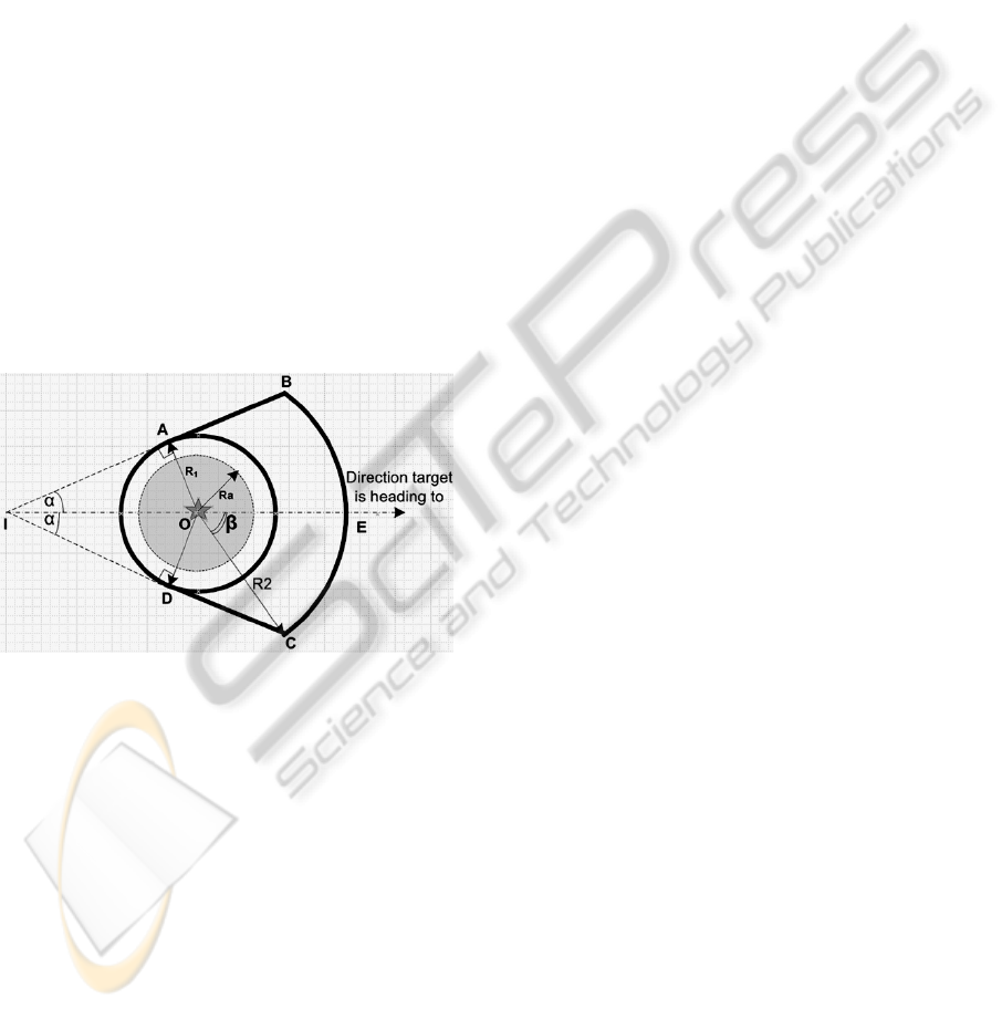
region R is defined by the circle radius
, the radius
of
and angle 2α – the region limited by the bold
line. R
2
, R
1
, and R
a
(R
2
> R
1
> R
a
) are activation
radius, sensing radius, and measurement radius
respectively. All the sensor nodes inside the region
of activation R are activated, while the nodes outside
the region are in sleep mode to save power. All the
nodes inside the circle (O, R
1
) can sense the target
while no node outside can detect the target.
However, only nodes inside the circle (O, R
a
) are
actively taking measurements and reporting the data
to the master node. This is done to account the
imprecision in the location information of a given
sensor node. For example, if there is 20%
uncertainty in measurement accuracy then the
solution R
1
=1.2R
a
can ensure that there are no
sensor nodes outside the circle (O, R
1
)
that can
detect the target . Assuming that the maximum
target velocity is known, and the direction of the
target does not change sharply. The selection of
R
2
=1.8R
a
and 2 60
can guarantee the sensors in
the moving direction of the target are activated in
advance. Thus, the WSN can track the target
continuously without any interruption.
Figure 1: The target represented by at point O. The
boundary of the region of activation R is limited by line
AB, curve BC, line CD and curve CA (the bold line
above). The curve BC is formed by part of the circle (O,
R
2
). No nodes outside circle (O, R
1
) can sense the target.
All the nodes inside R are activated. However, only the
sensors inside the circle (O, R
a
) are actively taking
measurement.
2.2 Settings
Initially, the sensor nodes in the boundary of the
field are on to detect intruders while the all other
sensors are off. If the maximum velocity of a target
is known, then the boundary nodes can turn on and
off periodically without losing the ability to track the
incoming target according to (Watfa, et al., 2006b).
When the boundary nodes detect an intruder, the
region R is formed and the nodes inside are
activated.
A master node is selected depending on two
criteria: the distance to the target and power residual.
The sensors inside the circle with radius R
a
take
measurements and transfer the measured data to the
master node. The master node runs the Kalman
Filter and obtains the estimated position and the
direction of the target. The master node broadcasts
the learned knowledge of the target to its neighbors.
After receiving the information, a node will turn on
or off depending on whether it is inside or outside
region R.
2.3 Position Calculation
After receiving the measurement from the target’s
neighbor sensor nodes, the master node uses the
trilateration and the least square algorithm to
calculate the position of the target.
Suppose there are k sensor nodes that are
actively taking measurements whose coordinates are
(x
1
, y
1
); (x
2
, y
2
); … (x
k
, y
k
), and measured distances
from each nodes to the target are d
1
, d
2
, … d
k
respectively.
The least square solution of the target’s
coordinate (x
t
, y
t
) is:
AbAA
y
x
T
t
t
1
)(
−
=
⎥
⎦
⎤
⎢
⎣
⎡
(1)
where A and b are in the following form:
⎥
⎥
⎥
⎥
⎥
⎥
⎦
⎤
⎢
⎢
⎢
⎢
⎢
⎢
⎣
⎡
−−
−−
−−
−−
=
−−
)(2)(2
)(2)(2
...
)(2)(2
)(2)(2
11
11
2323
1212
kk
kkkk
yyxx
yyxx
yyxx
yyxx
A
(2)
⎥
⎥
⎥
⎥
⎥
⎥
⎥
⎦
⎤
⎢
⎢
⎢
⎢
⎢
⎢
⎢
⎣
⎡
+−++−
+−++−
+−++−
+−++−
=
−−−
)()()(
)()()(
...
)()()(
)()()(
222
1
2
1
2
1
2
2
1
2
1
2222
1
2
2
2
2
2
3
2
3
2
3
2
2
2
1
2
1
2
2
2
2
2
2
2
1
kkk
kkkkkk
yxyxdd
yxyxdd
yxyxdd
yxyxdd
b
(3)
2.4 Power Consumption
The transmitted power
, received power
,
idle power
and sleeping power
are 1400 mW,
1000 mW, 830 mW, and 130 mW respectively based
on the power consumption analysis in (Watfa, et al.,
ICINCO 2010 - 7th International Conference on Informatics in Control, Automation and Robotics
56
2006b). From region R, the number of sensor nodes
inside the circle radius
is
.
is the number of
sensor nodes outside the circle with radius of
, but
inside the region R. The number of sensor nodes in
the sensor field and number of active sensor nodes in
the boundary are and
respectively. The total
power consumption of the sensor field in one
sampling cycle is calculated as owing. foll
The neighbors make
transmissions and
the master de r s
no eceives
time .
(4)
The master node broadcasts the target position
and its directions, and it makes one transmission.
Each of
neighbors in the cone area
receives the infor ation of t n .
m he target o ce
(5)
Each active node, except measurement nodes,
consumes an amo t energy unt of he idle
(6)
The other nodes are sleeping, and the total power
consum sed by these node is
(7)
Then to consu wer i
tal med po s
(8)
2.5 Distributed Kalman Filter
Local prediction (see (Rao, et al., 1991))
QkFkkPkFkkP
kkxkFkkx
T
+××=+
×=+
)()|()()|1(
)|(
ˆ
)()|1(
ˆ
(9)
Local update
)H(k)(kR)(kH(k|k)P|k)(kP
T
1111
111
+×+×++=+
−−−
)1()1()1()1(
1
+×+×+=+
−
kRkHkPkW
T
(10)
[
)|1(
ˆ
)1()1(
)1()|1(
ˆ
)1|1(
kkxkHkz
kWkkxkkx
+×+−+×
+
]
+
+=++
Where 1 is the target position calculated in
(1). The knowledge passed to the subsequent master
node
)1|1()1|1( ++++ kkPandkkx
3 NUMERICAL EXAMPLES
We will consider two scenarios to demonstrate the
distributed Kalman Filter for target tracking. In the
first, it is assumed that sensor nodes are uniformly
distributed. This requirement is relaxed in the
second scenario where the nodes are randomly
deployed. It is assumed that there is no hole in
coverage within the regions to be monitored, and
every point is covered by at least three sensors.
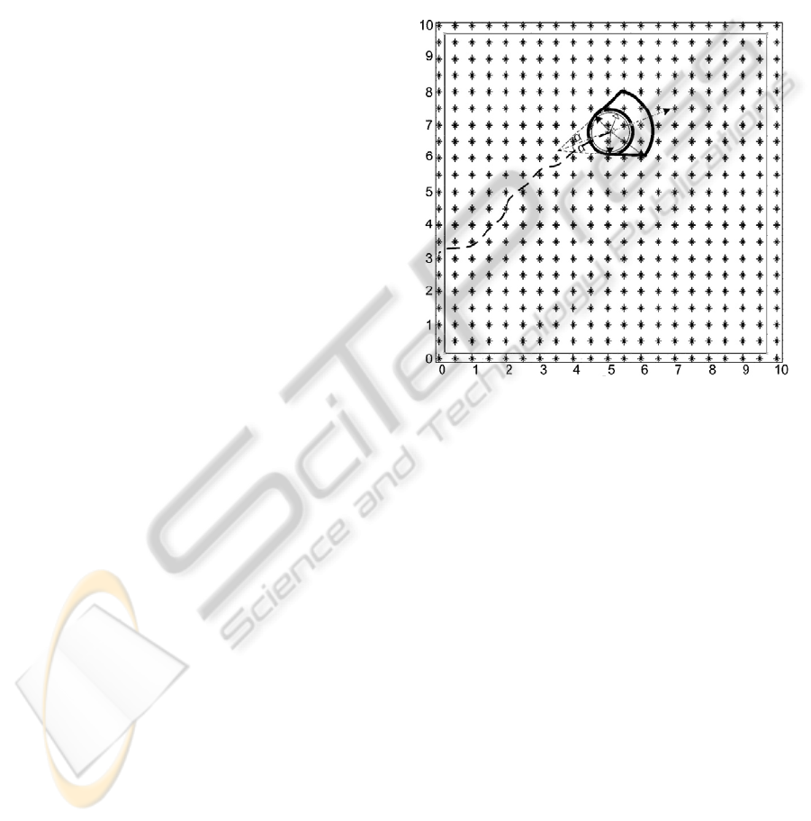
Figure 2: Example of sensor field and the trajectory of the
target. The sensor nodes in the boundary of the field are
always active. In the figure, all the nodes in the cone area
around the target are activated.
The sensor field is assumed to be a square of the
dimension 10 10 units as seen in Figure 2. By
choosing the distance of any two closest nodes is 0.5
units, the total number of uniformly distributed
sensor nodes is 441. The target is assumed to move
along the horizontal trajectory with the sinusoid
velocity profile while the vertical coordinate remains
at y = 5. In 10 seconds, the target travels between the
coordinates (0, 5) and (10, 5). The sampling
frequency is 200Hz and the simulation time is 10
seconds. The following difference equations are
used to model the dynamic behaviors of the moving
target.
(11)
Where
10
1
,
,
0 1
x
k
is the target velocity and and p
k
is target position
in x the direction at time k. Δt is the sampling time.
DISTRIBUTED KALMAN FILTER-BASED TARGET TRACKING IN WIRELESS SENSOR NETWORKS
57
Moreover, w
k
and v
k
are Gaussian distributed with
zero mean state noise and measurement noise. From
scenario 1 to scenario 4, the initial condition for the
Kalman Filter is the same as the true value while it is
nonzero in scenario 5. The sensor nodes are
uniformly deployed in scenario 1 to scenario 5 while
randomly deployed in scenario 6.
Scenario 1: Without using the Kalman Filter, more
sensors used in measurement results in better
estimated tracking. As seen in Table 1, when the
average measured sensor nodes increased from 4.5
to 17.5, the noise variance decreased from 21.71
10
to13.49 10
. However, the trade off is the
total power consumption of the network increases
from 1.38× 10
5
to 2.09× 10
5
(mW). The power
consumption analysis is shown in Figure 3.
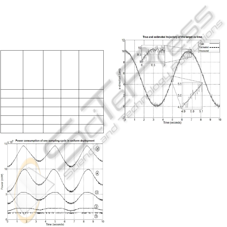
Table 1: Performance analysis.
Average
measured
sensors
Average
active
sensors
Error
variance
without
Kalman
lter Fi
Error
variance
with
Kalman
lter Fi
Average
total power
consumption
(10
-3
) (10
-3
) (mW × 10
5
)
4.5 9.3 24.71 3.63 1.38
17.5 39.2 13.49 1.57 2.09
60.4 139.9 7.03 0.98 4.48
130.8 275.5 4.62 0.31 7.88
279.1 416.2 5.43 0.10 12.60
Figure 3: Without the Kalman Filter, the line number 1, 2,
3, 4, and 5 have average measured sensor nodes of 4.5,
17.5, 60.4, 130.8, and 279 respectively. For the line
number 3 to 5, the total power consumption is fluctuated
because when the target moves close to the boundary the
number of active sensors is reduced. Then the total power
consumption reduces. Line #1 and #2 are quite flat
because in these scenarios the relatively small cone
regions result in small difference in the number of active
sensors when the target in the middle of the field and
when it is close to the boundary.
Scenario 2: When the Kalman Filter is used, the
variance of the estimated error is smaller and Figure
4 shows the smoother tracking performance
compared to scenario 1. As shown in Table 1, by
using the Kalman Filter, only an average of 4.5
measured sensors is sufficient to achieve the error
variance of 3.6310
which is smaller
than 5.43 10
resulted by an average of 279.1
measured sensors without using Kalman filtering.
Figure 4: Target's true trajectory is the solid black line,
and its estimations using trilateration with the Kalman
Filter and without the Kalman Filter are the solid gray line
and the dashed black line respectively. The average
number of measured sensors is 4.5, and the standard
deviation of state noise and measurement noise are 0.01
and 0.2 respectively. The Kalman Filter yielded both a
smaller error variance and smoother estimated trajectory.
As we zoom in two small sub figures, the estimated
position is close to the true position when the target moves
in a linear part of the sinusoid trajectory. Without using
the Kalman Filter, the estimated trajectory is noisy.
Scenario 3: When the number of average measured
sensors and the sampling frequency are fixed, slower
average velocity results in smaller estimated
tracking error as shown in Figure 5. In this scenario,
the sampling frequency is 200Hz, the standard
deviation of state noise and measurement noise are
0.01 and 0.2 respectively, and the average number of
measured sensors is 6.3.
ICINCO 2010 - 7th International Conference on Informatics in Control, Automation and Robotics
58
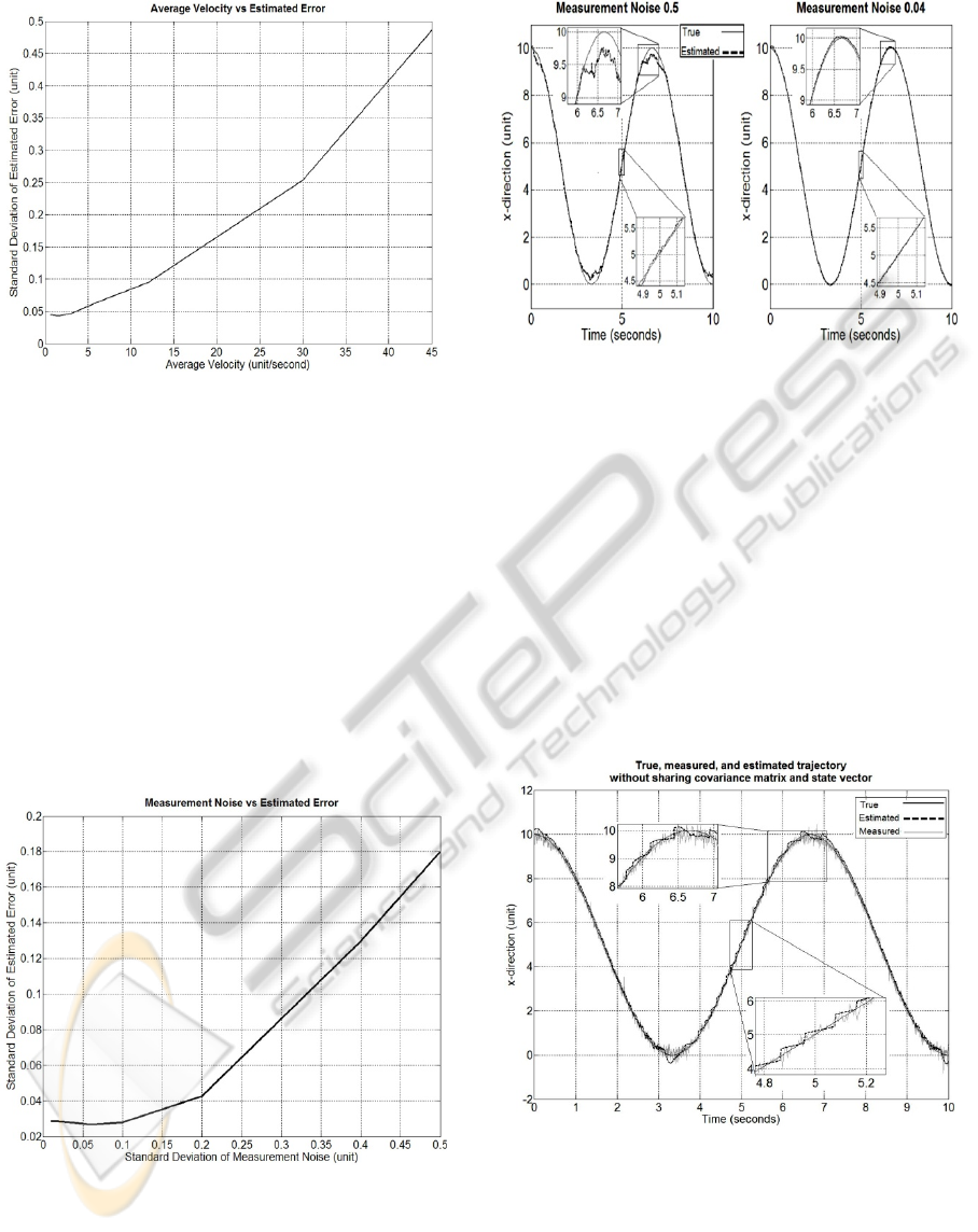
Figure 5: Average velocity increases as the estimated error
has a larger standard deviation.
Scenario 4: In this scenario, the sampling frequency
is kept at 200Hz, average target velocity is three
units per second and the average number of
measured sensors is 6.5. In Figure 6, the standard
deviation of state noise is fixed at 0.01 while the
measurement noise has a standard deviation varying
from 0.01 to 0.5. The variance of estimated error
increases with the increase in measurement noise. In
addition, with the same number of average measured
sensors of 6.5, the smaller measurement noise leads
to the better tracking performance. The tracking
performance, shown in Figure 7, is better when the
measurement noise is smaller.
Figure 6: When the distance measurement is subjected to a
larger noise, the variance of estimated tracking error
becomes bigger.
Figure 7: The true and the estimated trajectory with
different measurement noise levels. The standard
deviation of measurement noise is 0.5 in the left side while
it is 0.04 on the right side.
Scenario 5: When the master node does not share
the knowledge of the target including the target state
and the covariance matrix with the subsequent one,
the subsequent master node has to run the Kalman
Filter with the default initial conditions. Assuming
that the difference between the initial position and
the actual target position is the measurement error,
the change in master nodes is indicated by the abrupt
jumps in estimated error as shown in Figure 8. When
there is a change in the master node, the Kalman
Filter requires some extra time steps to converge.
Figure 8: Without sharing the state vector and covariance
matrix to the subsequently master node, each master node
has to start the Kalman Filter from scratch. The
measurement noise standard deviation is 0.2, while the
number of average measured sensor nodes is 7.6.
Scenario 6: As shown in Figure 9, when the sensor
nodes are randomly distributed, we get similar
results in comparison with the uniform scenario
DISTRIBUTED KALMAN FILTER-BASED TARGET TRACKING IN WIRELESS SENSOR NETWORKS
59

shown in Figure 3. However, the power
consumption is not as smooth as it is in the uniform
scenario. Due to the random nature, there are more
sensor nodes covering a specific point while fewer
sensor nodes are covering other points. In order for
our algorithm to work effectively, at least three
sensor nodes must cover each point in the sensor
field
Figure 9: Power consumption of one sampling cycle in
random deployment. There are 441 sensor nodes deployed
in the sensor field of 10 10. The line number 1, 2, 3, 4
and 5 have average measured sensors of 3.4, 15.7 59.5,
127.2, and 259.7 respectively.
4 DISCUSSIONS
The above results show that the distributed Kalman
Filter implementation in a WSN is successful in
tracking moving targets. The tracking error is small
when the target follows a linear trajectory while
nonlinear trajectories with high target velocities
result in higher tracking errors. However, in all these
scenarios, the tracking error is 12.5% smaller than
that obtained in the absence of the Kalman Filter. In
addition to the improved tracking performance, the
distributed filter requires fewer nodes to be active at
any given instant, thereby reducing the overall
power consumption of the WSN. This is significant
because the lowered power consumption increases
the useful life of the WSN.
The choice of the cluster head is determined by
the residual power (P
) of each node and its
distance to the target. At each instant, every active
node in the proximity of the target computes the
weighted sum of its residual power and its distance
to the target (D) as following
with constants α and β in the interval
0,1
. A node will become the new master node if
its weighted sum is smaller than that of the current
master node. Consequently, the knowledge of the
Kalman filtering is transferred from the current
master node to the new one.
5 CONCLUSIONS
In this paper, a method for the target tracking
problem using distributed Kalman Filter in WSNs is
demonstrated. The algorithm is robust to changes in
the velocity of the target and measurement noises.
The algorithm reduces the total power consumption
in the network in comparison with distributed
Kalman Filter algorithms elsewhere in literature.
Another contribution of the proposed algorithm is
the activation of a reduced set of sensor nodes for
target tracking. Thus, sensor nodes further away
from the target are inactive and thereby conserve
power. Fewer active nodes also mean reduced
communication among nodes. These two factors
together increase the useful life of the WSN while
provide accurate tracking in the presence of
measurement noise and target uncertainty.
The results presented in this paper assume that
each sensor node knows its position accurately and
share a common system clock with other nodes. This
is not a detriment as results in time synchronization
and localization already exist in the literature. Proof
of the convergence of the tracking error and the
stability of the overall system will be presented in an
extended version of the paper.
REFERENCES
Akyildiz, I. F., Su, W., Sankarasubramaniam, Y., &
Cayirci, E. (2002). A survey on sensor network, IEEE
Communications Magazine (Vol. 40 pp. 102-114).
Al-Karaki, J. N., & Kamal, A. E. (2004). Routing
techniques in wireless sensor networks: a survey.
Wireless Communications, IEEE, 11(6), 6-28.
Alriksson, P., & Rantzer, A. (2007, December 12-14 ).
Experimental Evaluation of a Distributed Kalman
Filter Algorithm. Paper presented at the 2007 46th
IEEE Conference on Decision and Control, New
Orleans, LA
Cardei, M., Thai, M. T., Li, Y., & Wu, W. (2005, March
13-17). Energy-efficient target coverage in wireless
sensor networks. Paper presented at the INFOCOM
2005. 24th Annual Joint Conference of the IEEE
Computer and Communications Societies, Miami,
Florida.
ICINCO 2010 - 7th International Conference on Informatics in Control, Automation and Robotics
60

Cattivelli, F. S., Lopes, C. G., & Sayed, A. H. (2008,
June). Diffusion strategies for distributed kalman
filtering: Formulation and performance analysis.
Paper presented at the Proc. 2008 IAPR Workshop on
Cognitive Information Processing, Santorini, Greece.
Chen, M., Gonzalez, S., & Leung, V. C. M. (2007).
Applications and design issues for mobile agents in
wireless sensor networks. IEEE Wireless
Communications, 14(6), 20-26.
Chiang, C., Wu, H., Liu, W., & Gerla, M. (1997, April).
Routing In Clustered Multihop, Mobile Wireless
Networks With Fading Channel. Paper presented at the
In Proc. IEEE SICON'97.
Hashemipour, H. R., Roy, S., & Laub, A. J. (1998).
Decentralized structures for parallel Kalman filtering.
IEEE Transaction on Automatic Control, 33(1), 88-94.
Intanagonwiwat, C., Govindan, R., & Estrin, D. (2000,
August). Directed Diffusion: A Scalable and Robust
Communication Paradigm for Sensor Networks. Paper
presented at the In Proceedings of the Sixth Annual
International Conference on Mobile Computing and
Networking (MobiCOM '00).
Kim, J.-H., West, M., Scholte, E., & Narayanan, S. (2008,
June 11-13). Multiscale consensus for decentralized
estimation and its application to building systems.
Paper presented at the 2008 American Control
Conference, Seattle, WA
Mutambara, G. O. (1998). Decentralized estimation and
control for multisensor systems: CRC Press.
Olfati-Saber, R. (2007, December 12-14). Distributed
Kalman filtering for sensor networks. Paper presented
at the 2007 46th IEEE Conference on Decision and
Control, New Orleans, LA
Olfati-Saber, R., & Shamma, J. S. (2005, December 12-
15). Consensus Filters for Sensor Networks and
Distributed Sensor Fusion. Paper presented at the 44th
IEEE Conference on Decision and Control, CDC-
ECC'05.
Rao, B. S., & Durrant-Whyte, H. F. (1991). Fully
decentralized algorithm for multisensor Kalman
filtering. IEE Proceedings-D Control Theory &
Application, 138(5), 413 - 420.
Uhlmann, J. K. (1996). General data fusion for estimates
with unknown cross covariances. Proceedings of
SPIE, 2755, 536-547.
Watfa, M. K., & Commuri, S. (2006a, August 14). The 3-
Dimensional Wireless Sensor Network Coverage
Problem. Paper presented at the 2006 IEEE
International Conference on Networking, Sensing and
Control. ICNSC '06, Ft. Lauderdale, FL.
Watfa, M. K., & Commuri, S. (2006b). Optimal sensor
placement for Border Perambulation. Paper presented
at the 2006 IEEE International Conference on Control
Applications, Munich, Germany.
DISTRIBUTED KALMAN FILTER-BASED TARGET TRACKING IN WIRELESS SENSOR NETWORKS
61
