SPATIAL KNOWLEDGE IN PLANNING LANGUAGE

Lamia Belouaer, Maroua Bouzid and Abdel-Illah Mouaddib

GREYC - CNRS (UMR0672), Universit

e de Caen, Basse-Normandie, ENSICAEN

Boulevard du Mar

echal Juin, 14032 Caen Cedex, France

Keywords:

Spatial representation and reasoning, Spatial ontology, Fuzzy information, Rules, Task and path planning.

Abstract:

This paper describes the integration of spatial knowledge in a planning problem. For example, in the case of

evacuation problem of a building during a ﬁre, we must know the fastest paths (the shortest, least congested,

. . . ). Such applications require spatial knowledge to perform spatial planning. This planning taste becomes

more complex when knowledge are shared by many actors. Indeed, our interest concerns collaborative work

between agents, in particular the case of human-robot interaction. In such contexts, considering the space

information in planning, we use a spatial ontology called SpaceOntology which handles different representa-

tions and abstraction levels of spatial information. We integrate this ontology in the planning by deﬁning a

formal language planning: Spatial-PDDL. Spatial-PDDL combines PDDL concepts with this ontology. Also,

we distinguish between three types of actions: non spatial, spatial and navigation actions.

1 INTRODUCTION

In this paper, we focus on the spatial knowledge man-

agement in planning problem where the tasks con-

sider spatial and non-spatial representations. Such

problems could be met in human-robot interaction.

Most typical scenarios include a human instructing

a robot to perform some actions on some objects in

the environment. To achieve this task, the human and

the robot establish a similar description of the con-

cerned environment. This requires not only that the

scene descriptions created by the robot and the human

match but also needs a system which can success-

fully mediate between these descriptions. However,

the space representation from human’s and robot’s

points of view is not the same. Indeed, the robot’s

spatial representation is numeric and the human’s spa-

tial representation uses natural language. The natural

language employs incomplete and fuzzy information

about space (for example, the book is near the bottle).

Thus, we propose to ﬁnd a representation for planning

problems that can be used by robots to communicate

with humans, analyze scenes and build maps.

To do this, we use an ontology called SpaceOn-

tology (Belouaer et al., 2010). It permits a knowl-

edge representation for modeling space, spatial rela-

tions and fuzzy information. This ontology allows us:

a complex spatial description, an easy management of

various spatial aspects, an easily extensible structure

and to infer spatial information. It provides a struc-

tured knowledge about the environment to explore in

planning process.

Planning process in artiﬁcial intelligence is deci-

sion making about the actions to be taken. As input,

this process takes a planning problem (initial state and

goal state) returns a plan (a sequence of ordered ac-

tions) to solve this problem (achieve the goal state

from the initial state). To express spatial knowledge

in planning process, we need a formal language. We

use language PDDL (Ghallab et al., 1998) (Planning

Domain Deﬁnition Language).

We propose a planner incorporating spatial rep-

resentation and reasoning by integrating SpaceOntol-

ogy. SpaceOntology in the planning, is not used for

veriﬁcation or control, but as information needed for

planning. We adapt the PDDL actions and concepts

deﬁnition to express spatial information if it is nec-

essary. In other words, we extend PDDL to spatial

knowledge: Spatial-PDDL.

The rest of paper is organized as follows. Sec-

tion 2 gives an overview about different approaches

to solve planning problems taking spatial knowledge

into account. Section 3 describes the spatial repre-

sentation and reasoning. Section 4 describes the plan-

ning process with spatial knowledge and its impact on

complexity. Section 5 presents some results. Finally,

we conclude in Section 6.

Belouaer L., Bouzid M. and Mouaddib A..

SPATIAL KNOWLEDGE IN PLANNING LANGUAGE.

DOI: 10.5220/0003654400710080

In Proceedings of the International Conference on Knowledge Engineering and Ontology Development (KEOD-2011), pages 71-80

ISBN: 978-989-8425-80-5

 2011 SCITEPRESS (Science and Technology Publications, Lda.)

2 RELATED WORK

Different techniques for spatial representation and

reasoning have been proposed. Most are based on

constraints, logical and algebraic approaches (Bal-

biani et al., 1999). However, these approaches can not

manage numeric, topological and imprecise knowl-

edge at the same time. In planning, we need to com-

bine these knowledge. Thus, we must use an uniﬁed

framework to cover large classes of problems and to

give rise to instantiations adapted to each particular

application. Ontologies appear as an appropriate tool

toward this aim.

Spatial ontologies can be found in some ﬁelds

such as Virtual Reality (Dasiopoulou et al., 2005),

Robotics (Dominey et al., 2004), etc. All these on-

tologies are focused on the representation of spatial

concepts according to the application domains. A

major weakness of usual ontological technologies is

their inability to represent and to reason with impreci-

sion. An interesting work presented in (Hudelot et al.,

2003) overcomes this limit.

The concept of exploiting ontology to represent

spatial knowledge in planning has been explored.

(Bouguerra et al., 2008) describes a new approach

for monitoring the execution of plans where spatial

knowledge is deﬁned by an ontology called LOOM.

This ontology permits a region classiﬁcation and ver-

iﬁes the plan execution. However, it does not describe

spatial relations and it is not used in planning.

To express spatial knowledge in planning process,

we use PDDL (Ghallab et al., 1998). The ﬁrst version

of PDDL is extended to consider several aspects in a

planning problem deﬁnition that improve the quality

of the solution, such as the temporal dimension (Fox

and Long, 2003). Despite the importance of the spa-

tial dimension in planning problem, PDDL with spa-

tial deﬁnition is not yet integrated.

Our main contribution is the extension of PDDL to

spatial knowledge: Spatial-PDDL. To do this, we use

SpaceOntology that considers several spatial knowl-

edge aspects; the space hierarchy, spatial relations

(numeric, topological and fuzzy).

3 SPATIAL REPRESENTATION

AND REASONING

In the following, we present SpaceOntology (Be-

louaer et al., 2010), a framework for spatial represen-

tation and reasoning.

3.1 Spatial Representation

We opted for OWL

(Baader, 2003) as a formal

language

. An important characteristic of DL is its

expressivity and its capability of inferring knowledge

from the known information.

Regions

HasRelation

WithIntersection

Thing

TopologicalRelations

VerticalRelations HorizontalRelations

FuzzyDistance

NumericDistance

DistanceRelations

Space

SpatialRelations

AxisRelations

HasRelation

Figure 1: Graphical representation of SpaceOntology.

A spatial entity is described by two concepts

Regions and Space. The concept Space (Spacev

Thing) is used to model space: the name of places,

the hierarchical level, the boundaries deﬁnition, etc.

It represents a global environment (a country, a city,

a building, . . . ). The concept Regions (Regionsv

Space) is a sub-space included in a given space. A

region is itself considered as a space that can be de-

composed into different sub-regions. From a geomet-

ric point of view, a region rg is deﬁned by the small-

est rectangle rect corresponding to its axis-aligned

bounding rectangles. These concepts include some

attributes. The hierarchical space organization has an

impact on the distance evaluation. Indeed, the dis-

tance of 10 meters in a city is considered as close,

however in a corridor this distance is considered as

far. Each region has the attributes alpha and beta

depending on the scale of its level. These two pa-

rameters evaluate the distance between two spatial ob-

jects (Belouaer et al., 2010) (section 3.2.3).

A spatial relation is deﬁned by the concept

SpatialRelations (SpatialRelationsv Thing)

which includes TopologicalRelations and

DistanceRelations. A spatial relation is a

concept on its own. A Topological relation

(TopologicalRelations) is an ABLR rela-

tion (Laborie et al., 2006). This relation is a couple

, r

i, where: r

∈ {L, O

, I

, O

, R} and

∈ {A, O

, I

, O

, B}. A Distance relation

(DistanceRelations) can be an Euclidean distance

(NumericDistance) between the symmetry points

of two rectangles representing two regions (r referent

object and ε target object) noted d(ε, r) (in R

)

Web Ontology Language

Description Logics

All notations used here are deﬁned in the DL.

KEOD 2011 - International Conference on Knowledge Engineering and Ontology Development

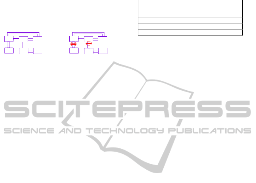
Figure 2: Graphical illustration of SpaceOntology to describe structures in speciﬁc domains.

or fuzzy distance (FuzzyDistance) evaluating a

distance between the symmetry points of two rect-

angles representing two regions. A fuzzy distance

is deﬁned by four linguistic variables: close to,

close enough, far enough and far.

To deﬁne a spatial relation between spatial enti-

ties, we use the concept HasRelation. This concept

links with a spatial relation between a reference re-

gion and one or more target regions (Example 1).

There are several relations (or predicates) to link

these concepts to provide a spatial semantic. For ex-

ample to express a hierarchical relation between two

regions, we consider the links:

• consistsOf:

Space v Thing u ∃ consistsOf.Regions

u > 1 consistsOf

• isPartOf:

Regions v Space u ∃ isPartOf.Space

u > 1 IsPartOf

Example 1. Let us consider a part of a ﬂoor with two

ofﬁces (O1, O2) and a hall (H1) (Fig. 3).

Figure 3: Partial Map.

Figure 2 models

the space domain deﬁned in

Figure 3 by using SpaceOntology. We consider that

each spatial entity is a Regions concept. Then, spa-

tial relation between these different spatial entities

are described by combining SpatialRelations and

HasRelation.

For more readability, we omit certain classes and at-

tributes.

In Example 1, the relation1 is an instance of the

concept HasRelation describing the topological re-

lation between ofﬁces O2 and O1:

relation1:HasRelation

u ∃ concernsSpatialRelation.inside below

u ∃ hasReferent.O1 u ∃ hasTarget.O2

The relation inside below is deﬁned as follow:

inside below:TopologicalRelations

u ∃ isAnHorizontalRelation.I

u ∃ isAVerticalRelation.B

3.2 Spatial Reasoning

The reasoning methods infer spatial information in

order to enrich the description of the environment

and/or to manage the lack of information.

3.2.1 Spatial Hierarchical Reasoning

To express a hierarchical relation between two re-

gions (for example, a region includes another region,

or a region is in another one), we use the predicates

consistsOf and isPartOf. The predicate isPartOf

is the inverse of the relation consistsOf. These rela-

tions are transitive. The transitivity rules for the pred-

icate consistsOf and isPartOf are:

consistsOf(r 1,r 2) u consistsOf(r 2,r 3)

−→ consistsOf(r 1,r 3)

isPartOf(r 1,r 2) u isPartOf(r 2,r 3)

−→ isPartOf(r 1,r 3)

To consider a space as a whole with the different

abstraction levels is not always necessary and makes

spatial reasoning very expensive. The hierarchical or-

ganization can simplify this reasoning, depending on

abstraction level. To do so, we exploit the two pred-

icates: consistsOf and isPartOf in order to deﬁne

the function hierarchical interest zone denoted Z

(r).

SPATIAL KNOWLEDGE IN PLANNING LANGUAGE

This function Z

(r) deﬁnes an interest zone (An in-

terest zone deﬁnes a region in a considered space to

be reached and/or localized) of a region r in the hier-

archical level l. To compute this function we query

SpaceOntology (details in Section 4.2.1).

3.2.2 Spatial Reasoning based on Topological

Relations

In order to enrich SpaceOntology with new knowl-

edge, we consider two different aggregations of spa-

tial relations: combination ⊕ and composition ⊗.

The Combination Mechanism. The combination

concerns topological relations. As mentioned, a topo-

logical relation is a couple hr

, r

i. This mechanism

consists of combining horizontal relation r

with ver-

tical one r

( r

⊕ r

). This mechanism is deﬁned

by a set of rule proposed in SpaceOntology. Rules

deﬁnition for the combination mechanism is used in

order to deﬁne the 36 topological relations of ABLR

(Neighborhood graph (Laborie et al., 2006)), dynam-

ically. These relations express topological relations

(overlaps, touch, . . . ) and orientation relations. In-

deed, by this mechanism we can represent the 8 car-

dinal relations (left, above, above left, . . . ) and other

directional relations as at the same level, between, etc.

Figure 4 presents a rule which allows the combination

of the horizontal relation L(Le f t) and the vertical re-

lation A(Above).

isATopologicalRelation(?t relation)

u isAVerticalRelation(?t relation,"A")

u isAnHorizontalRelation(?t relation,"L")

−→ is(?t relation,"left above")

Figure 4: Rule deﬁnition for left above.

The Composition Mechanism. The composition

mechanism infers new spatial information. Let us

consider three regions deﬁned by three rectangles

rect1, rect2 and rect3. The idea is to infer which re-

lation R3 links between rect1 and rect3 where R1 is a

relation between rect1 and rect2 and R2 is a relation

between rect2 and rect3. The topological relation R

is deﬁned by R3 = R1 ⊗ R2, then

hrx3, ry3i = hrx1, ry1i ⊗ hrx2, ry2i (1)

= hrx1 ⊗ rx2, ry1 ⊗ ry2i (2)

The composition results of (rx1 ⊗ rx2) and (ry1 ⊗

ry2) are given by the composition table of rectangle

algebra by preserving the directionality property as

deﬁned in ABLR. Formally, we deﬁne in SpaceOn-

tolgy a set of rules reﬂecting the composition table.

The composition mechanism returns a disjunction of

possible relations between two rectangles. However,

not all inferred relations are valid. To reduce the num-

ber of possible relations between two rectangles, by

keeping only the valid relations, we proceed as fol-

lows. First, we select the necessary knowledge for the

inference and we formalize it as a constraint network

called spatial relation network. Then, we apply the

required rules, and we complete this network. Thus,

a network is deﬁned by :

• V a set of nodes representing rectangles describ-

ing regions,

• C a set of constraints representing topological re-

lations. An arc is labeled by a topological relation

(constraint) between two rectangles connected to

this arc. Arcs labeled with disjunctions are arcs

that are inferred by composition.

The idea is to remove all spatial relations does

not ensure the consistency of the network. Thus, we

aim to establish arc consistency in this network. We

produce an equivalent network to the ﬁrst one which

checking the arc consistency property (Def. 1).

Deﬁnition 1. A network is arc consistent if all its arcs

are arc consistent

Thus, the network produced is arc-consistent, i.e.

it does not contain topological relations does not en-

sure the arc consistency of the network. Practically,

for the rules application, we use the Pellet inference

engine (Sirin et al., 2007), and for the veriﬁcation

of the arc consistency, we rely on the MAC algo-

rithm (Prosser, 1995).

Example 2. Let us consider the following problem,

a robot is in the ofﬁce o2. Its mission is to go to the

ofﬁce o3 . However, it has no spatial information en-

abling it to deﬁne its trajectory between o2 and o3.

Figure 5: Spatial Relation Between o1 and o3.

We have a set of spatial information, depicted

in Figure 5: the ofﬁce o3 is right and is overlaps

above the ofﬁce o1: o3hR, O

io1. Also, in Figure 3,

the ofﬁce o2 is inside and is below of the ofﬁce o1:

o2hI

, Bio1.

Our goal is to found the spatial relation between

the ofﬁces o3 and o2. First, we apply a symmetry rule,

then, o1hL, O

io3 is the inverse of o3hR, O

io1. Sec-

ond, we apply composition rule between o2hI

, Bio1

and o1hL, O

io3 (Fig. 6).

Thus, from this information we can plan our tra-

jectory to reach the ofﬁce o3 without considering

KEOD 2011 - International Conference on Knowledge Engineering and Ontology Development

translate(?link,?t link) u translate(?relation, ?t relation) u concerns(?link,?relation)

u hasTarget(?link,?tgt) u hasReferent(?link,?ref) u isANumericDistance(?relation)

u isPartOf(?ref,?region) u isPartOf(?tgt,?region)

u swrlb:greaterThan(distanceValue(?relation),0)

u swrlb:lessThanOrEqual(distanceValue(?relation),alpha(?region))

−→

[concerns(?t link,?t relation) u hasTarget(?t link,?tgt) u hasTarget(?t link,?tgt)

u hasReferent(?t link,?ref) u isAFuzzyDistance(?t relation) u is(?t relation,"close")]

Figure 7: Rule Deﬁnition of Def close relation.

isATopologicalRelation(?t relation1)

u isAnHorizontalRelation(?t relation1,"I X")

u isAVerticalRelation(?t relation1,"B")

u isATopologicalRelation(?t relation2)

u isAnHorizontalRelation(?t relation2,"L")

u isAVerticalRelation(?t relation2,"O B")

−→ [isATopologicalRelation(?t relation3)

u isAnHorizontalRelation(?t relation3,"L")

u isAVerticalRelation(?t relation3,"B")]

Figure 6: Rule deﬁnition for left below with composition.

the entire second ﬂoor but only the northeastern part

of the ﬂoor from the ofﬁce o2. The information

o2hL, Bio3 is added in SpaceOntology.

3.2.3 Spatial Fuzzy Reasoning

In this work, the fuzzy representation concerns only

distance relations. Indeed, we use linguistic variables

to evaluate a distance (close, close enough, far enough

and far). We aim to give a numeric representation to

each variable and vice versa. SpaceOntology allows

this translation, by deﬁning some rules based on func-

tions N

α,β

and F

α,β

(Schockaert, 2008). The function

(α,β)

(p, q) (resp. F

(α,β)

(p, q)) measures the degree

with which p is close to q (resp. the degree with which

p is far from q) (α, β > 0).





d(p,q)

 , 

 p ,q

 , 

 p , q

Figure 8: Distance evaluation. (1) if d ∈ [0, α] , then d is

close , (2) if d ∈]α, α +

] then d is close enough, (3) if

d ∈]α+

, α+β] then d is far enough, (4) if d ∈]α+β,+∞[

then d is far.

Figure 8 illustrates the translation of a distance

from a numeric deﬁnition to symbolic deﬁnition and

vice versa. The parameters α and β allow us to eval-

uate the numeric distance. These parameters depend

on the current region. Figure 7 is a rule allowing us to

evaluate a distance relation.

The rule Def

close relation (ﬁg. 7) translates a

numeric distance (NumericDistance) (distanceValue

(?relation)) in symbolic evaluation (FuzzyDistance)

given by the instance close which indicates the close

relation. This rule is apply for distance (distanceValue

(?relation)) between 0 and α.

4 SPACEONTOLOGY BASED

PLANNING

Now, we explore the potential uses of spatial repre-

sentation and reasoning offered by SpaceOntology in

planning. Our goal is to propose a planner incorpo-

rating spatial representation and reasoning: Spatial

Planner (Fig. 9).

domain

initial state

goal

a2 an

....

plan

Planner

task planner

path planner

SpaceOntology

Figure 9: Spatial Planner.

As input, the spatial planner (Fig. 9) takes a plan-

ning problem deﬁned by:

• a domain is a set of actions. Each action speciﬁes

preconditions that must be present in the current

state so it can be applied, and effects on the current

state,

• a description of the initial state of a world,

• a description of a goal.

As output, it generates a plan: a sequence of actions.

This planner consists of a task planner and a path

planner and SpaceOntology. The task planner’s aim

is to deﬁne the sequence of actions which will be ex-

ecuted to achieve the goals of the entry problem. Path

planner deﬁnes possible paths to reach the execution

of tasks to accomplish. It ﬁnds a path between two

positions (fuzzy positions or well deﬁned positions).

SpaceOntology manages spatial information about the

space.

There is a communication between these compo-

nents (Fig. 9). This communication is in the form of

queries/answers. These one is in charge of planners

which at some steps require spatial preconditions to

be satisﬁed. To this end, it sends a query to SpaceOn-

tology to answer to the request.

SPATIAL KNOWLEDGE IN PLANNING LANGUAGE

Example 3 (Study Case). A team (human and robot)

is in the ofﬁce O

in the ﬁrst ﬂoor of the building B

(the human position is h) (Fig.10). The human asks

the robot to pick up a book (b) located in the ofﬁce (o)

close to the coffee machine. This machine is on the

second ﬂoor of the building B

(Fig.10).

Figure 10: Abstract Map.

Figure 11: Deadlocks.

The robot’s goal is to fulﬁll this mission. A clas-

sical task planner provides: (1) go-to(o

,o), (2)

take(b), (3) go-to(o,h), (4) give(b) as a plan.

Several problems requiring spatial information are

identiﬁed: (1) in which position the robot should exe-

cute an action ( go-to(o

,o)). The ofﬁce o is de-

ﬁned as the ofﬁce close to the coffee machine, i.e.

how to evaluate the relation close to the coffee ma-

chine? (2) how to move between different areas to ac-

complish actions? i.e to deﬁne the robot’s navigation

during and between each action; for example, ﬁnding

a path between the current position o and the human

position h. (3) how to order the action execution with

respect to navigation?

To solve this problem, we use the Spatial Plan-

ner (Fig. 9). This planner requires different types of

knowledge encoded in Spatial-PDDL. It is an exten-

sion of PDDL with spatial information made by the

communication between planners (task and path plan-

ner) and SpaceOntology (Fig. 9). We focus here on

Spatial-PDDL deﬁnition and the planner operation.

4.1 From PDDL to Spatial-PDDL

We extend PDDL with spatial knowledge using

SpaceOntology in order to improve the expressiveness

of the planning language. Formally, SpaceOntology is

a triple (Φ, R, I), where Φ is a set of concepts, R is a

set of relations (or predicates) between concepts and

I is a set of instances which depends on the described

environment.

Our planner takes three inputs (Fig. 9). (1) An ini-

tial state S

, (2) a goal state S

; these states describe a

set of objects (O) by specifying their type (T ) and re-

lations between them (Π), (3) A set of actions (A) de-

scribed in a domain (D). We extend PDDL language

with SpaceOntology.

4.1.1 Notations

The main extensions are summarized in Table 1.

Table 1: Extended Notions with SpaceOntology Elements.

Notions PDDL Extend PDDL with SpaceOntology

Predicate Π Π ← Π ∪R

Type T T ← T ∪ Φ

Domain D use of extends and @ns

Objects O spatial/non spatial objects

Actions A non spatial/spatial/navigation actions

A concept, a relation or an instance always has

a preﬁx. (Dou, 2008) expresses that the domain is

extended by an ontology, where the notion of “ :

extends” and “@ns1 : ” were introduced. Each con-

cept in SpaceOntology deﬁnes a spatial type. All

the concepts deﬁned in SpaceOntology (Φ) are intro-

duced and exploited for extending PDDL (Table. 1).

A predicate π (π ∈ Π) expresses a relation. All the re-

lations (R) deﬁned in SpaceOntology are introduced

and exploited for extending PDDL (Table. 1).

Our contributions concerning the action deﬁni-

tion consist of the extension of geometric precondi-

tions/effects in order to take the different spatial rep-

resentations (topological and fuzzy information) into

account. In addition, it consists of the deﬁnition of the

spatial fuzzy actions (Def. 2).

Deﬁnition 2 (A Spatial Fuzzy Action). A spatial

fuzzy action a is deﬁned by a = ( at , pr,

q, e) , where : at, pr and e are respectively pa-

rameters for the action, preconditions, effects as de-

ﬁned in the extended action (Guitton, 2010) and q is

a set of queries.

Example 4. The semantic of the action take

(Fig. 12) is: the robot r takes the book b located in

the ofﬁce deﬁned in a fuzzy way ?o. The ofﬁce ?o

is deﬁned in Spatial-PDDL as a query variable (Dou,

2008).

take(r,b,?o)

(robot r) (book b)(empty-arm r)

(¬(has r b))(region ?o)(At r ?o)

(:query

(freevars (?o - Region ?α ?β -@xsd:int

?rel - SpatialRelations ?hr - HasRelation)

(and(@ns:isPartOf ?o Z

Level(C M )−1

(CM ))

(@ns:hasTarget ?hr ?o)(@ns:hasReferent ?hr CM)

(@ns:concernsRelation ?hr ?rel)

(if(instanceOf ?rel NumericDistance)

(and(owl:DatatypeProperty rdf:ID="α" ?α Z

Level(C M )

(CM ))

(owl:DatatypeProperty rdf:ID="β" ?β Z

Level(C M )

(CM ))

(bounded-int owl:DatatypeProperty rdf:ID="distance" ?α (?α+ ?β))))

(if(instanceOf ?rel FuzzyDistance) (= ?rel "close_to")))))

(At r p

)(@ns:isPartOf p

?o)

(bounded-int distance(p

r.arm , b), ?α

, ?β

)

(:query

(freevars (?α

?β

-@xsd:int)

(and(owl:DatatypeProperty rdf:ID="α" ?α

?o)

(owl:DatatypeProperty rdf:ID="β" ?β

?o))))

(frontOf r.arm, b) (sameLevel r.arm,b)

(¬(empty-arm r) (has r b)

Figure 12: Modeling the Action take in Spatial-PDDL.

To delimit this region, we query SpaceOntology

(details in Section 4.2.1). The fuzzy relation close

can be described in a numeric way. So, we seek an

KEOD 2011 - International Conference on Knowledge Engineering and Ontology Development

ofﬁce satisfying the fuzzy relation close by translat-

ing it in a numerical representation (Belouaer et al.,

2010). Moreover, the action execution requires that

the precondition (At r p

) is satisﬁed. However, the

satisfaction of this precondition requires the deﬁnition

of the position p

. This position is deﬁned as follows.

First, it must be in the ofﬁce ?o. Then, it must al-

low us to reach the target; the book. This requires

that the robot is at a position p

close to the book.

The evaluation of this distance is made by the func-

tion bounded-int. Also, there are two functions like

frontOf and sameLevel which must be satisﬁed in

order to grab the book.

4.1.2 Integrating SpaceOntology in PDDL:

Spatial-PDDL

We translate any spatial knowledge described in

SpaceOntology to the domain and problem deﬁnitions

in PDDL. SpaceOntology has an open world assump-

tion and PDDL a closed one. To overcome this difﬁ-

culty, the translation concerns only known types.

Our model requires as an input : (1) a planning

domain describes each action of a system in Spatial-

PDDL, (2) a planning problem describing the initial

state and goals in Spatial-PDDL, (3) SpaceOntology

gives spatial description of space, and (4) some re-

quired information.

Deﬁnition 3 (A Domain). A planning domain D =

(A, Π), where A = {a

, a

, . . . , a

} a set of actions,

where a

is an action and Π set of relations between

objects O.

Deﬁnition 4 (A Spatial Planning Problem). A Spatial

Planning Problem P = < O, S

, S

>, where O is a

set of spatial and non-spatial objects, S

is an initial

state that could be associated to fuzzy position and

is the goal state that could be associated to fuzzy

position.

In Figure 13, some objects are spatial (:regions

CM ?o), others are non spatial (:objects

human robot book). The initial state expresses an

initial symbolic situation human has not the book

(not (has human book)). Also, it expresses the

initial spatial situation the robot is in the ofﬁce O

(At robot O

Note by “?α” and “?β” query variables to deter-

mine the α and β of the current level. The relation

owl:DatatypeProperty rdf:ID="β" identiﬁes for

a given region the β (Fig. 13).

The fuzzy spatial information the ofﬁce close to

the coffee machine is deﬁned by a query variable:

“?o”. There are some functions. (distance?ip?t p −

position) used to compute the Euclidean distance

between two positions. (maxhdistance) (resp.

(define (problem bookmissionpb)

(:domain bookmission)

(:objects

Arnaud - human

Bobo - robot

book table - item

o11b1 - region

?target - region ;; fuzzy region)

(:init

(on book table)

(At Arnaud o11b1)

(At Bobo o11b1)

(At table ?target)

(Empty Arnaud)

(Empty Bobo)

(= (maxhdistance) 1)

(= (minhdistance) 0.5)

(not (Holding Arnaud book)

)

(:query

(freevars (?target - region ?α ?β -@xsd:int)

(and ( In ?target Z

Level(cm)−1

(cm)

(owl:DatatypeProperty rdf:ID="α" ?α Z

Level(cm)

(cm))

(owl:DatatypeProperty rdf:ID="β" ?β Z

Level(cm)

(cm))

(bounded-int distance(?o, cm) ?α (?α+ ?β)))))

)

(:goal ( and

(not(on book table))

(Holding Arnaud book))))

Figure 13: An Example of Spatial-PDDL Problem.

(minhdistance)) indicates the maximum distance

(resp. minimum) from which the interaction with hu-

mans can not be executed. path (Fig. 14) checks the

existence of a path and computes it.

(define (domain bookmission)

(:requirements :typing :fluents)

(:extends

(uri ".../SpaceOntology.owl" :prefix sponto))

(:types actor - object

item - object

human robot - actor)

(:spatial-types region - @sponto:Regions)

(:predicates (Empty a - actor)(Holding a - actor i - item)

(on i - item t - item)))

(:spatial-predicates (At o - object p - region))

(:functions (distance ip tp - position)(maxdist)(mindist)

(maxhdist)(minhdist)(path irg trg - region))

(:action go

:parameters(r - robot irg - region trg - region )

:precondition (and(At r irg)(not(At r trg)))

:spatial-precondition (=(path irg trg)true))

:effect(and(At r trg) (not(At r irg))))

(:action pick-up ...)

(:action put-down ...)

(:action give ...)

(:action take ...))

Figure 14: An Example of Spatial-PDDL Domain.

4.2 Communication between

Components

The planner has three components: task planner, path

planner and SpaceOntology. The communication be-

tween them is in form of request/response. Planners

(task and path) formulate queries to spatial ontology.

They are encapsulated in the preconditions of the ac-

tions or they are directly in the problem deﬁnition.

SPATIAL KNOWLEDGE IN PLANNING LANGUAGE

In this section, we start by specifying the types of

queries necessary for the planner function. Then, we

describe the operation.

4.2.1 Requests for SpaceOntology

Several types of queries that are needed for the system

operation. We can classify them into three categories:

Adjacency query, Proximity Query and Hierarchi-

cal Interest Zone Query

Adjacency Query. We assume that each region is

adjacent to its neighbors with access points (doors,

intersection of corridors, . . . ) called gates. A gate

allows transitions between adjacent regions (in the

same hierarchical level or in different hierarchical lev-

els). A gate allows us to connect more than two re-

gions.

Two regions are adjacent if there is a/or a set of

transition between these two regions. Two types of

adjacency: direct adjacency (i.e, the longer of the

path between these two regions is equal to 1 (number

of gates), of course several possibilities may exist, this

represents a multiple choice of paths) and indirect ad-

jacency (i.e, the longer of the path between these two

regions is more than 1 (number of gates))

To extract the gates between regions or neigh-

bors for a given region, we use adjacency query to

SpaceOntology.

SELECT ?referent ?target "

WHERE {"?x ns:label ?relation."

"?x ns:hasintersection \"gate\"."

"?x ns:hasReferent ?referent. "

"?x ns:hasTarget ?target."}

This query takes as parameter a gate (gate) and

deﬁnes the regions connected to this gate. The indi-

rect adjacency is inferred by the existence of a path

(of length greater than one see next section).

Proximity Query. A proximity query deﬁnes re-

gions that are close to a given region or if a region

is near or far from another region.

SELECT ?referent ?target "

WHERE {"?x ns:concerns \"close\"."

"?x ns:hasReferent ?referent. "

"?x ns:hasTarget ?target."}

This query takes a parameter relation (close) and

deﬁnes the regions that are close.

Hierarchical Interest Zone Query. To deﬁne the

function Z

(r), we deﬁne the hierarchical interest

zone query.

SELECT * "

WHERE {"?region rdf:type ns:Regions ."

"?region ns:label \"" + rg +"\" ."

"?region ns:isPartOf ?father . "

"?father ns:level ?level." }

"Filter ( ?level = " + level + " ).

This request is used to return the area of interest

for the region rg level hierarchical level.

4.3 Spatial Planning Process

During the selection of these actions, the planner

asks the satisfaction of these preconditions using

SpaceOntology. Then, it calculates the required dis-

placements and returns an answer to the result thereof.

If the navigation is possible so action can be executed.

Otherwise another action must be found to achieve the

mission. The execution of the action take the book

(Fig. 12) requires that the robot is in the ofﬁce close to

the coffee machine (in which the book is). However,

the robot is in another ofﬁce : O

. Thus, a naviga-

tion between the current position and target position

is required. The target position is deﬁned in a fuzzy

way. Formally, we assume that the general planning

problem includes a fuzzy path planning problem.

Deﬁnition 5 (Fuzzy Path Planning Problem.). Let us

consider two fuzzy positions (

) and a spatial de-

scription given by SpaceOnology (Φ, R, I). A path so-

lution Pth between

is a continuous sequence of

positions/regions that allows the robot to move from

the initial state to the goal state while avoiding obsta-

cles.

4.3.1 Path Planning

Our main contributions to the path planning focus

on using space hierarchy, topological spatial relations

and spatial fuzzy information.

Let us consider that the initial position i

is ac-

curate

and the target position

is fuzzy. The path

planning operation is detailed in the following.

Generation of Crossing Network Graph. A

Crossing Network Graph Γ

is a directed graph.

Nodes are organized hierarchically. Edges represent

hierarchical relation between nodes. A node in this

graph represents a Crossing Network or a region.

Deﬁnition 6 (Crossing Network Γ). A graph Γ =

(V ,E), where; V = (v

, . . . , v

) is a set of vertices, each

is a crossing network and E = (e

, . . . , e

) is a set of

To simplify the explanation, the initial position is crisp.

This work may well be applied in the context of precise

positions.

KEOD 2011 - International Conference on Knowledge Engineering and Ontology Development

edges, each e

deﬁnes an adjacency relation, a gate-

way and a congestion.

Each element of Crossing Network Graph is re-

lated to the mission. This graph deﬁnes all possible

paths between ip and

t p.

Example 5. In example 3, the team is in ofﬁce O

and the target is in ﬂoor E

. These ofﬁces are not in

the same hierarchical level. In addition, these regions

and E

) are not adjacent. Thus, ﬁnding a path

between these two regions exploits the space hierar-

chy and adjacency links deﬁned in SpaceOntology.

Level 1

Level 2

Level 3

d21

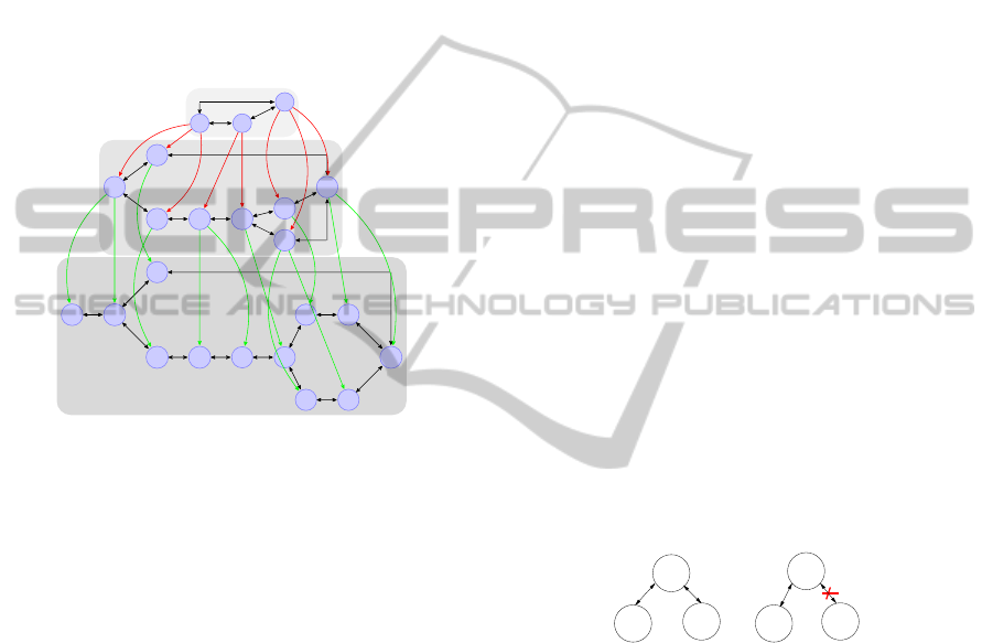
Figure 15: Crossing Network Graph.

First, we consider the most abstract regions for

and E

in the same level, there are B1 and B6.

Then, we look for the adjacency links between B1

and B6. We assume that each region is adjacent to

its neighbors with gates. To extract gates between

regions, we query the ontology. So, we generate all

possible paths between buildings B1 and B6 by con-

sidering B2 ,B3, B4 and B5. However, the passing

through the buildings B2, B4 and B5 is not neces-

sary (Fig. 11). For B2 and B5 they are not included

in the mission; they are a deadlocks regions (one gate

to exit/entrance). For B4, it is not included in the mis-

sion. Also, this region is connected to a deadlock re-

gion B5. So, B4 is also a deadlock region. By combin-

ing all these concepts we generate a directed graph:

Crossing Network Graph (Fig. 15). Nodes are orga-

nized hierarchically. Edges represent hierarchical re-

lation between nodes. A node in this graph represents

a Crossing Network (a graph given the adjacency rela-

tions between regions in the same hierarchical level).

Each node of one level l is developed until reaching

the target hierarchical level. We assume that N

is a

subset of regions in the level l. E

is a set of edges.

Edges represent spatial adjacency relations between

two nodes giving gateways. For each n ∈ N

, n must

satisfy the selection criteria.

Path Computing. We search a path between two

positions i

(accurate position) and

(fuzzy position)

in the Crossing Network Graph, based on two crite-

ria measures (Mouaddib, 2004): (1) minimize the Eu-

clidean distance between i

and

and (2) facilitate

access to a region, to ensure fast and simple actions.

We combine these concepts in order to improve the

path solution quality. These criteria, allow the robot

to execute its actions in an easy and quick way (the

choice of paths that are short in terms of distance)

and to maintain the speed of navigation. We deﬁne

a measure: Θ(p

, p

) = (d(p

, p

), c(p

, p

)), where

d(p

, p

) is the euclidean distance between p

et p

and c(p

, p

) measures the congestion in the region

between p

and p

. Pathﬁnding in crossing network

graph consists of path search in crossing network for

each hierarchical level. A path solution is a sequence

of paths pth

, . . . , pth

, where pth

contains nodes of

the i-th level and that are a specialization of nodes on

pth

i−1

(i.e the path solution in level 1 is B1−C6 −B6,

the pathﬁnding in level 2 will not consider the sub

nodes of the node B3 (Fig. 15). In each level, we

use multi-criteria Dijkstra’s algorithm with a single

source Z

). It returns the shortest path between the

source node and the target one Z

(

) (i is the abstract

level). The shortest path is the path minimizing the

measure Θ

= (d, c)

, where d is the Euclidean dis-

tance and c is a congestion measure. In order to min-

imize Θ

, we compute it as described in (Mouaddib,

2004): Θ

∑

crit∈{d,c}

Regret(crit). The concept is

to minimize the regret (Fig. 16).

E2 E3

c1(3,5)

c2(0,9)

c1(3,5)

c2(0,9)

(0,5)*

Figure 16: Regret Based Path Selection.

We compute θ

∗

, where this measure is θ

∗

(0, 5)

∗

= [Min(3, 0), Min(5, 9)]. Then, for each edge

e, we compute the distance between θ

∗

and θ

Min(Dist) =



Dist(θ

, θ

∗

) = Dist((3, 5), (0, 5)) = 3

Dist(θ

, θ

∗

) = Dist((0, 9), (0, 5)) = 4

Finally, we select the edge allowing us the mini-

mum distance with θ

∗

: edge c

(Fig. 16).

We are not interested in the global network in level

i. Indeed, we consider that the nodes and edges be-

longing to the path solution of level i − 1. We can

generate the path for each node in the next level and

exploit the hierarchical aspect of space which reduces

the search time. Indeed, only nodes of the at level i

are extended in level i + 1 and thus some edges in the

graph are not explored.

SPATIAL KNOWLEDGE IN PLANNING LANGUAGE

5 EXPERIMENTS

We present some experimental results to solve plan-

ning described with Spatial-PDDL.

5.1 Experimental Results

The computation time to solve a spatial planning

problem described in Space-PDDL depends on com-

puting time of answering to queries.

Table 2: Computation Time of Plan Solution Generation

Solving the problem in Example 3 (seconds). The path

computation time is less then one second.

Queries Solving

problemQueries number Answer to query

[2-8] < 1 < 1

[9-13] [1-2.2] [1 - 3.08]

[14-20] [3.01-4.8] [4.01 - 7]

[21-30] [5.05-10.09] [8.07 -

15.01]

Table 2 shows that the computation time depends

on the number of requests and the response time.

The latter depends on the rules number deﬁned in

SpaceOntology. This computing time is very reason-

able even if we have a large number of requests. In-

deed, in Table 2, for a query number between 21 and

30, solving the problem is done in 15.01 seconds.

6 CONCLUSIONS

Our main contribution was the extension of PDDL to

spatial knowledge: Spatial-PDDL. To do this, we uses

SpaceOntology that considers several spatial knowl-

edge aspects; the space hierarchy, spatial relations

(numeric, topological and fuzzy). This permits to

consider not only numeric spatial information in pre-

conditions but also topological and fuzzy information.

Moreover, spatial reasoning (the inference mecha-

nisms) provided by this ontology permits a complex

reasoning. SpaceOntology in the planning, is not used

for veriﬁcation or control, but as information needed

for planning.

Future work will concern the improvement of spa-

tial interaction between human and robots. In other

words, we aim to formalize communication between

them, especially in the case where the set of fuzzy

rules are not sufﬁcient to ﬁnd a solution.

REFERENCES

Baader, F. (2003). The description logic handbook: theory,

implementation, and applications. Cambridge Univ

Pr.

Balbiani, P., Condotta, J.-F., and del Cerro, L. F. (1999). A

new tractable subclass of the rectangle algebra. IJCAI.

Belouaer, L., Bouzid, M., and Mouaddib, A. (2010). On-

tology based spatial planning for human-robot inter-

action. TIME.

Bouguerra, A., Karlsson, L., and Safﬁotti, A. (2008). Mon-

itoring the execution of robot plans using semantic

knowledge. Robotics and Autonomous Systems.

Dasiopoulou, S., Mezaris, V., Kompatsiaris, I., Papastathis,

V., and Strintzis, M. (2005). Knowledge-assisted se-

mantic video object detection. IEEE Transactions on

Circuits and Systems for Video Technology.

Dominey, P., Boucher, J., and Inui, T. (2004). Building

an adaptive spoken language interface for perceptually

grounded human–robot interaction. In IEEE-RAS/RSJ

international conference on humanoid robots.

Dou, D. (2008). The Formal Syntax and Semantics of Web-

PDDL.

Fox, M. and Long, D. (2003). PDDL2. 1: An extension

to PDDL for expressing temporal planning domains.

JAIR.

Ghallab, M., Howe, A., Knoblock, C., McDermott, D.,

Ram, A., Veloso, M., Weld, D., and Wilkins, D.

(1998). PDDL the planning domain deﬁnition lan-

guage. AIPS.

Guitton, J. (2010). Architecture hybride pour la planiﬁca-

tion d’actions et de dplacemen.

Hudelot, C., Atif, J., and Bloch, I. (2003). Fuzzy spatial

relation ontology for image interpretation. Fuzzy Sets

and Systems.

Laborie, S., Euzenat, J., and Layaıda, N. (2006). A spatial

algebra for multimedia document adaptation. SMAT.

Mouaddib, A.-I. (2004). Multi-objective decision-theoretic

path planning. In ICRA.

Prosser, P. (1995). Mac-cbj: maintaining arc consistency

with con ict-directed backjumping. Research report,

177.

Schockaert, S. (2008). Reasoning about fuzzy temporal and

spatial information from the web. PhD thesis, Ghent

University.

Sirin, E., Parsia, B., Grau, B., Kalyanpur, A., and Katz, Y.

(2007). Pellet: A practical owl-dl reasoner. Web Se-

mantics: science, services and agents on the World

Wide Web, 5(2):51–53.

KEOD 2011 - International Conference on Knowledge Engineering and Ontology Development