IMPACT OF WINDOW LENGTH AND DECORRELATION STEP ON

ICA ALGORITHMS FOR EEG BLIND SOURCE SEPARATION

Gundars Korats

1,2

, Steven Le Cam

and Radu Ranta

CRAN UMR 7039 Nancy Université, CNRS, 2 Avenue de la Forêt de Haye, 54516, Vandoeuvre-les-Nancy, France

Ventspils University College, 101 Inzenieru iela, LV-3601, Ventspils, Latvia

Keywords:

EEG, BSS, ICA, Whitening, Sphering.

Abstract:

Blind Source Separation (BSS) approaches for multi-channel EEG processing are popular, and in particular

Independant Component Analysis (ICA) algorithms have proven their ability for artifacts removal and source

extraction for this very speciﬁc class of signals. However, the blind aspect of these techniques implies well-

known drawbacks. As these methods are based on estimated statistics from the data and rely on an hypothesis

of signal stationarity, the length of the window is crucial and has to be chosen carefully: large enough to get

reliable estimation and short enough to respect the rather non-stationary nature of the EEG signals. In addition,

another issue concerns the plausibility of the resulting separated sources. Indeed, some authors suggested

that ICA algorithms give more physiologically plausible results depending on the chosen whitening/sphering

step. In this paper, we address both issues by comparing three popular ICA algorithms (namely FastICA,

Extended InfoMax and JADER) on EEG-like simulated data and assessing their performance by using an

original correlation matrices distance measure and a separation performance index. The results are consistent

and lead us to a precise idea of minimal sample size that guarantees statistically robust results regarding the

number of channels.

1 INTRODUCTION

The analysis of electro-physiological signals gener-

ated by brain sources leads to a better understanding

of brain structures interaction and are useful in many

clinical applications or for brain-computer interfaces

(BCI) (Schomer and Lopes da Silva, 2011). One of

the most commonly used method to collect these sig-

nals is the scalp electroencephalogram (EEG). The

EEG consists in several signals recorded simultane-

ously using electrodes placed on the scalp (see ﬁg.1).

The electrical activity of the brain sources is in fact

propagated through the anatomical structures and the

resulting EEG is a mixture (with unknown or difﬁ-

cult to model parameters) of brain sources and other

electro-physiological disturbances, often with a low

signal to noise ratio (SNR) (Sanei and Chambers,

2007).

The blind source separation (BSS) is a nowa-

days well established method to solve this problem,

as it can estimate both the mixing model and origi-

nal sources (Cichocki and Amari, 2002). In particu-

lar, approaches based on High Order Statistics (HOS)

such as Independent Component Analysis (ICA) are

common methods in this context and have been very

useful for denoising purpose or brain sources identi-

ﬁcation. However, the performances of these algo-

rithms are highly dependent on their pre-conditioning

given by 1) the data length chosen regarding the num-

ber of channels, and 2) the necessary decorrelation

step on which they are based. In this paper we eval-

uate the sensitivity to this pre-conditioning for three

popular ICA algorithms based on HOS: FastICA, Ex-

tended InfoMax and JADER.

1) The use of BSS on EEG signals implicitly as-

sumes that the estimated statistics are meaningful.

In order to ensure the reliability of these statistics,

different authors propose optimal sample sizes (i.e.

EEG signal time points), generally equal to k × n

where n is number of channels and k is some em-

pirical constant varying from 5 to 32 (Särelä and Vi-

gario, 2003; Onton and Makeig, 2006; Delorme and

Makeig, 2004). If these assumptions are correct, large

amount of channels requires huge sample sizes, pro-

cessing and time resources. On the other hand, EEG

signals are at most short term stationary, so it would

be interesting to ﬁnd a sufﬁcient inferior bound for

the number of necessary samples. The ﬁrst question

is then how to deﬁne a minimum sample size that

provides reliable estimation of sources and mixing

Korats G., Le Cam S. and Ranta R..

IMPACT OF WINDOW LENGTH AND DECORRELATION STEP ON ICA ALGORITHMS FOR EEG BLIND SOURCE SEPARATION.

DOI: 10.5220/0003780000550060

In Proceedings of the International Conference on Bio-inspired Systems and Signal Processing (BIOSIGNALS-2012), pages 55-60

ISBN: 978-989-8425-89-8

 2012 SCITEPRESS (Science and Technology Publications, Lda.)

model.

2) A second question addressed in this paper con-

cerns the stability (robustness) of the BSS results. As

it will be explained in the next sections, BSS includes

an optimization step. The results of this optimiza-

tion to some algorithms might depend on the initial-

ization of the algorithm. In the EEG and BSS litera-

ture (Palmer, 2010), some authors observed that using

different initializations (different decorrelation meth-

ods like classical whitening or sphering), the results

are more or less biologically plausible (thus implic-

itly different). The second auxiliary objective of this

paper is then to evaluate the statistical robustness of

several well known BSS algorithms to the initializa-

tion (decorrelation) step.

2 PROBLEM STATEMENT

2.1 EEG Mixing Model

Classical EEG generation and acquisition model is

presented in Figure 1. It is widely accepted that the

signals collected by the sensors are linear mixtures of

the sources (Sanei and Chambers, 2007).

Figure 1: EEG linear model.

Subsequently, the EEG mixture can be written as

X = AS, (1)

where X are the observations (electrodes), A is the

mixing system (anatomical structure) and S are the

original sources.

2.2 EEG Separation Model

We restrain in this paper to classical well determined

mixtures, where the number of channels is equal to

the number of underlying sources. In this case, BSS

gives the linear transformation (separating) matrix H

and the output signal vector Y = HX, containing

source estimates. Ideally, the global system matrix

G = HA between the original sources S and their es-

timates Y will be a permuted scaled identity matrix,

as it can be proven that the order and the original am-

plitude of the sources cannot be recovered (Cichocki

and Amari, 2002).

In all BSS methods, the matrix H is obtained as

a product of two statistically based linear transforms:

H = JW with

• W performing data orthogonalization: whiten-

ing/sphering,

• J performing data rotation : independence maxi-

mization via higher-order statistics (HOS) or joint

decorrelation of several time (frequency) intervals

The ﬁrst step (data decorrelation) can be seen as an

initialization for the second step. In theory any or-

thogonalization technique can be used to initialize the

second step but in this paper we will focus on two

popular decorrelation techniques: whitening (classi-

cal solution) and sphering (assumed to be more bio-

logically plausible (Palmer, 2010)).

2.2.1 BSS Initialization: Whitening/Sphering

Whitening. In general EEG signals X are correlated

so their covariance Σ will not be a diagonal matrix and

their variances will not be normalized. Data whiten-

ing means projection in the eigenspace and normali-

sation of variances. The whitening transform can be

computed from the covariance matrix of the data X

(assumed zero-mean): Σ = E{XX

Write the eigen-decomposition of Σ as

Σ = ΦΛΦ

, (2)

with Λ the diagonal matrix of eigenvalues and Φ the

eigenvectors matrix. Eigenvectors form a new or-

thogonal coordinate system in which the data are pre-

sented. The matrix Φ thus diagonalizes the covari-

ance matrix of X. Final whitening is obtained by sim-

ply multiplying by scale factor Λ

−

= Λ

−

X. (3)

After (3), the signals are orthogonal and with unit

variances (4) (Figure 2(c)).

} = I. (4)

Sphering. Data sphering completes whitening by

rotating data back to the coordinate system deﬁned

by principal components of the correlated data (Fig-

ure 2(d)). We can say that sphered data are turned as

close as possible to the observed data. To estimate the

sphering matrix we only need to multiply the whiten-

ing matrix with the eigenvector matrix Φ (Vaseghi and

Jetelová, 2006)

sph

= ΦΛ

−

X. (5)

BIOSIGNALS 2012 - International Conference on Bio-inspired Systems and Signal Processing

(a) Original sources (b) Mixed data

Figure 2: Example of different decorrelation approaches for

two signals

2.3 Optimization (Rotation)

Second step would be ﬁnding a rotation matrix J

to be applied to the decorrelated data (whitened or

sphered) in order to maximize their independence.

Rotation can be done using second order statistics

(SOS) using joint decorrelations and/or using HOS

cost functions. We restrain here to the second (HOS)

approach

. Several cost functions and optimization

techniques were described in the literature (see for

example (Cichocki and Amari, 2002; Delorme and

Makeig, 2004)). Among the most well known and

used in EEG applications, we can cite FastICA (neg-

entropy maximization (Hyvärinen, 1999)), Extended

InfoMax (mutual information minimization (Bell and

Sejnowsky, 1995)) and JADE/JADER (joint diagonal-

ization of fourth order cumulant matrices (Smekhov

and Yeredor, 2004)).

Speciﬁcally, in this paper we test the performances

and the robustness of the three cited ICA algorithms

with respect to the sample size and the initialization

step.

As described in the next section, in our simulations

we used random non-Gaussian stationary data, without any

time-frequency structure. Therefore algorithms based on

SOS as SOBI, SOBI-RO and AMUSE were not used.

3 PERFORMANCE EVALUATION

CRITERIA

3.1 Reliable Estimate of the

Covariance: Riemannian

Likelihood

As noted before, BSS model consists of decorrelation

and rotation. Both steps are based on statistical es-

timates. The ﬁrst step is common for all algorithms

and relies on the estimation of the covariance matrix.

Therefore it is necessary to have reliable estimates of

this matrix. In other words, given a known covariance

matrix Σ, we want to evaluate the minimum sample

size m necessary to obtain a covariance matrix estima-

tion

close enough to the original one with respect

to a distance that we have to deﬁne.

We propose here an original distance measure be-

tween the true and the estimated covariance matrices,

inspired from digital image processing and computer

vision techniques (Wu et al., 2008). In the context

of object tracking and texture description, a distance

measure is used to estimate whether an observed ob-

ject or region corresponds to a given covariance de-

scriptor. To estimate similarity between matrices re-

spectively corresponding to the target model and the

candidate, and knowing that covariance matrices are

symmetric positive deﬁnite, the following general

distance measure can be used:

(

, Σ) = tr



log



−



(6)

An exponential function of the distance is adopted as

the local likelihood

p(Σ

) ∝ exp{−λ · d

(Σ,

)}. (7)

In all the test procedures reported in this paper, we

ﬁxed the parameter λ to the constant value λ = 0.5 as

proposed in literature (Wu et al., 2008). This p(Σ

)

value varies between 0 and 1, 1 meaning perfect esti-

mation (Σ =

). A p(Σ

) value of 0.95 is considered

as a well chosen threshold above which the covariance

matrices are considered to be equal.

3.2 Separability Performance Index

In order to measure the global performance of BSS al-

gorithms (orthogonalization plus rotation), we use the

performance index (PI) (Cichocki and Amari, 2002)

deﬁned by

on Riemannian manifolds

IMPACT OF WINDOW LENGTH AND DECORRELATION STEP ON ICA ALGORITHMS FOR EEG BLIND

SOURCE SEPARATION

PI =

2n(n − 1)

∑

i=1

∑

j=1

i j

max

− 1

2n(n − 1)

∑

j=1

∑

i=1

i j

max

k j

− 1

(8)

where g

i j

is the (i, j)-element of the global system

matrix G = HA, max

| is the maximum value

among the absolute values of the elements in the ith

row of G and max

k j

| is the maximum value among

the absolute values of the elements in the jth column

of G. When perfect separation is achieved, the per-

formance index is zero. In practice a PI under 10

−1

means that the separation result is reliable.

4 RESULTS AND DISCUSSION

4.1 Simulated Data

Simulated EEG was obtained by mixing simulated

sources. We have chosen to simulate stationary white

source signals, as the retrieval of time structures is not

the purpose of this work (in fact, in all the tested al-

gorithms, as in most of the HOS type methods, the

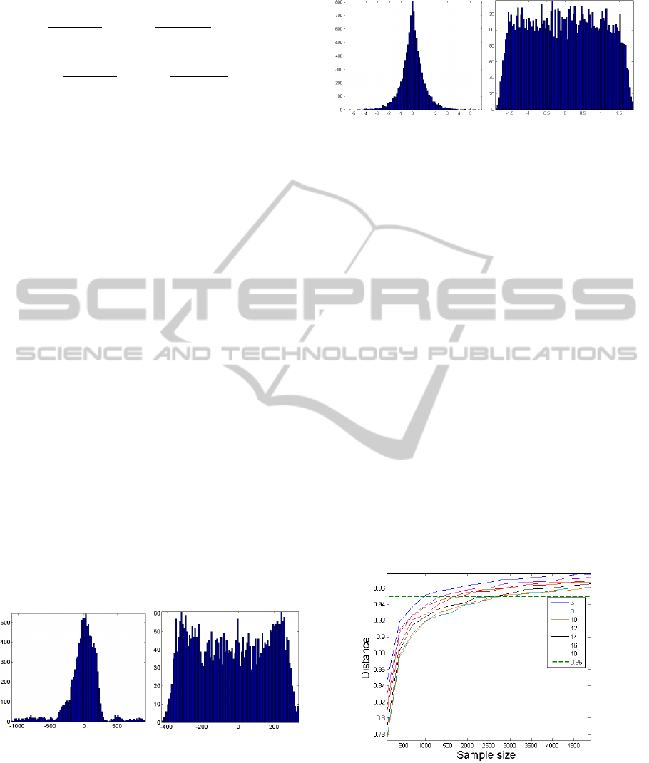
time structure is ignored). In order to have realistic

distributions of the sources, we analysed depth intra-

cerebral measures (SEEG). According to our observa-

tions (see also (Onton and Makeig, 2006; Särelä and

Vigario, 2003)), the distribution of the electrical brain

activity signals can be suitably modelled by General-

ized zero-mean Gaussians, as shown in ﬁg. 3(a) and

ﬁg. 3(b)). For this reason we randomly generated both

supergaussian (Laplace - Figure 4(a)) and subgaus-

sian (close to uniform (Figure 4(b))) distributions.

(a) Normal background (b) Oscillatory signal

Figure 3: Histograms of two SEEG samples.

Several simulations were made, using 6, 12 and

18 source signals. Half of the sources were gener-

ated as supergaussian and half as subgaussian. The

sources were afterwards mixed using a randomly gen-

erated mixing matrix A whose values vary in the

range [−1, ..., 1]. We then consider here the perfor-

(a) Supergaussian data (b) Subgaussian data

Figure 4: Histograms of generated data.

mance of each of the three ICA algorithms facing sim-

ulated stationary non-artefacted data.

One could argue that more realistic contexts

should have been simulated by using head models,

realistic neural sources and extra-cerebral artefacts in

order to generate the simulated channels. As the pur-

pose here is the determination of a minimum amount

of data needed for a reliable source separation in

favourable conditions (after an artefact elimination

step for example), we decided to use stationary ran-

domly mixed data for gaining more generality.

4.2 Reliable Estimate of the Covariance

This section presents the results of the covariance es-

timation robustness vs the length of the data. The dis-

tance between covariance matrices was computed us-

ing 6 from different sample sizes starting from 100

points till 5000 points. The likelihood was further

evaluated using 7. A constant threshold was empir-

ically ﬁxed to p = 0.95 (Figure 5): likelihood values

above this threshold are assumed to guarantee good

estimation of covariances as stated in section 3.1.

Figure 5: Riemannian likelihood for different sample sizes.

Each curve corresponds to a different number of channels

(from 6 to 18). The threshold p = 0.95 is displayed as a

dotted line.

As it can be seen in Figure 6, this estimate is be-

tween the bounds given in the literature, close to the

upper bound (30n

) for low number of channels n but

BIOSIGNALS 2012 - International Conference on Bio-inspired Systems and Signal Processing

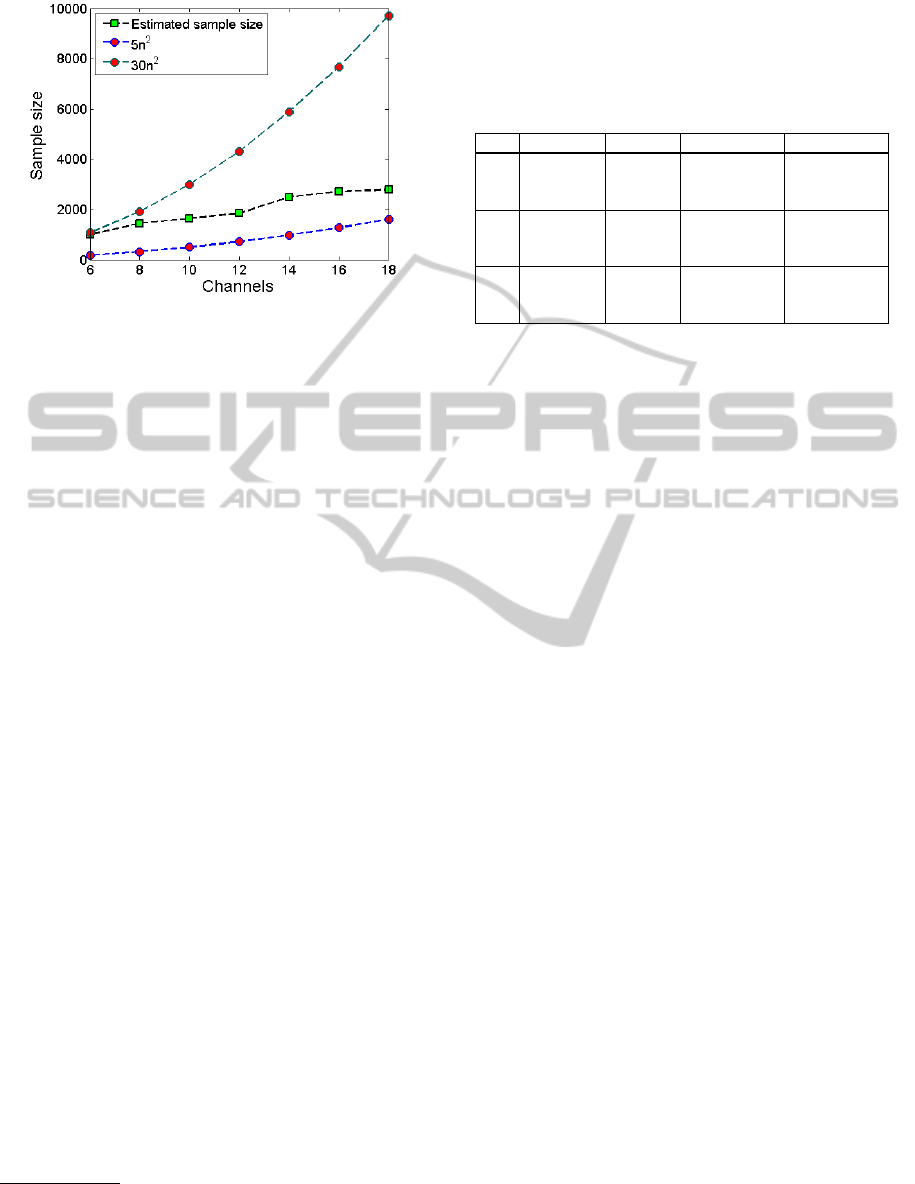
Figure 6: Sample size vs. number of channels for the pro-

posed decision rule (likelihood = 0.95).

increasing much slower. A possible way to interpret

the ﬁgure 6 is to use it as a decision rule: for a given

number of channels, one can estimate the minimum

number of data points necessary to have a reliable es-

timate of the covariance matrix and thus a reliable

whitening. This decision rule leads to data lengths

of about 1800 for 12 channels (2800 for 18 channels)

data points, that is about 7s (11s respectively) for a

sampling rate of 256 Hz. This range of time length

is more compatible with the stationarity hypothesis

than the values obtained using the 30n

rule (Delorme

and Makeig, 2004; Onton and Makeig, 2006). Indeed,

with this rule, we get 4320 (17s) and 9720 (38s) data

points respectively for 12 and 18 channels, which is

rather contradictory (at least in a realistic EEG setup)

with the assumption of stationarity on which BSS al-

gorithms are based

. As the next step (namely opti-

mization step) of the three considered algorithms is

based on HOS, these results are not sufﬁcient to as-

sess good separation results. Next section discusses

the validity of the ﬁnal unmixing results regarding the

data length given by the decision rule described in this

section.

4.3 Separability Performance

The global performances of ICA algorithms are here

evaluated using the PI given by (8). For the number

of points determined using the previous empirical rule

based on the covariance estimate (Riemannian likeli-

hood) and for different number of channels, the PI is

computed for each algorithm, the results being pre-

sented in table 1. We present two sets of results, ob-

tained considering either classical whitening or spher-

ing as the ﬁrst decorrelation/initialization step. Recall

This observation is important especially for high reso-

lution EEG measures, when the number of channels can be

very high.

that our second objective was to assess the sensitivity

of the ICA algorithms to this initialization.

Table 1: PI values (mean and standard deviation) for differ-

ent number of channels and different ICA algorithms using

whitening (PI

) or sphering (PI

)

Ch Methods Length PI

± STD PI

± STD

FastICA

1000

0.102±0.02 0.104±0.02

EI-MAX 0.381±0.17 0.417±0.13

JADER 0.095±0.02 0.093±0.02

FastICA

1800

0.082±0.01 0.082±0.01

EI-MAX 0.359±0.13 0.349±0.13

JADER 0.072±0.01 0.074±0.01

FastICA

2800

0.067±0.01 0.067±0.01

EI-MAX 0.284±0.10 0.327±0.07

JADER 0.059±0.01 0.059±0.01

From Table 1 we conclude that separation perfor-

mance are satisfactory for FastICA and JADER as the

PI are close or below the threshold value of 0.1 for

every amount of channels considered. This reinforce

the validity of the empirical rule given by the results

section 4.2. In addition, according to table 1, PI val-

ues indicate better performances when the number of

channels is increasing with respect to our empirical

rule. This could suggest that our proposed criterion

could be relaxed and the number of points could be re-

duced further. But, on the other hand, one must take

into account that these tests are performed on simu-

lated stationary random data: if outliers are present,

HOS estimates are more affected than the SOS es-

timations that used to deﬁne our threshold, thus a

higher amount of points might be needed for HOS re-

liable estimation.

We have to notice here that in all simulations Ex-

tended InfoMax seems to provide worse results than

the two other tested algorithms, conﬁrming the results

presented in (Ma et al., 2006). This phenomenon ap-

pears because of our choice of the simulated data. In-

deed, because of the use of subgaussian sources, the

algorithm (even in the extended version) needs more

data points in order to give reliable results. The evo-

lution of the PI for this algorithm, as a function of

the length of the data, is displayed in Figure 7. Em-

pirically, one can say that the 30n

rule seems to be

adapted for the Extended InfoMax algorithm, but ap-

parently too strong for the two others.

Table 1 allows to conclude also that each algo-

rithm is showing similar separability performance re-

gardless of the decorrelation step (whitening or spher-

ing). As it was expected, the optimization step is

then not sensitive to the initialization point set by the

decorrelation step for this kind of simulated stationary

non artefacted data. It would be interesting to test fur-

ther the robustness of these ICA algorithms when fac-

ing more realistic EEG like data. Such a study would

come to conﬁrm or inﬁrm the assumption made in a

IMPACT OF WINDOW LENGTH AND DECORRELATION STEP ON ICA ALGORITHMS FOR EEG BLIND

SOURCE SEPARATION

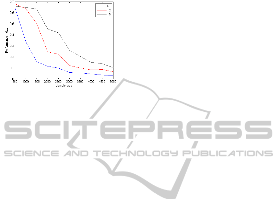
Figure 7: Extended InfoMax PI evolution for different num-

ber of channels as a function of the data length.

previous work (Palmer, 2010) stating that, for EEG

signals, using sphering instead of classical whitening

would result in more physiologically plausible sepa-

rated sources (i.e. more dipolar).

5 CONCLUSIONS AND FUTURE

WORK

Three popular ICA algorithms, often used to anal-

yse EEG signals, have been tested for different data

lengths and number of signals. The main objective

was to deﬁne a low bound of data length for robust

separation results, in order to take into account the

short term stationarity of the EEG signals. The re-

sults on simulated mixtures of subgaussian and su-

pergaussian sources are signiﬁcant enough to extract

an empirical rule for the minimum data length, de-

pending on the number of channels. This result is

based on an original distance measure inspired by the

computer vision community and leads to a reasonable

time length (approximately 10s for 18 channels, sam-

pled at 256 Hz). An auxiliary objective was to test the

convergence robustness of these algorithms for differ-

ent initializations (whitening or sphering). Separation

Performance Index turns out to be similar whether

the decorrelation step is performed using sphering or

whitening method, conﬁrming the robustness of these

algorithms.

Still, these results are not sufﬁcient to conclude

on the impact of different decorrelation methods on

real EEG signals. We are considering further work on

EEG-like (dipolar mixtures) simulated data corrupted

with noise, in order to evaluate the importance of the

decorrelation step from a physiological point of view

(source dipolarity). If such sensitivity is conﬁrmed,

a longer term ambition would be to ﬁnd an adequate

decorrelation scheme that guarantees the convergence

of ICA algorithms to plausible physiological sources.

Finally, an immediate perspective would be to

extend our study to more HOS algorithms and

more channels, but also to use more realistic time-

structured data allowing the evaluation of SOS BSS

algorithms (SOBI and similar).

REFERENCES

Bell, A. and Sejnowsky, T. (1995). An information-

maximization approach to blind separation and blind

deconvolution. Neural Computation, 7(6):1129–1159.

Cichocki, A. and Amari, S.-I. (2002). Adaptive Blind Signal

and Image Processing. Wiley-Interscience.

Delorme, A. and Makeig, S. (2004). EEGLab: an

open source toolbox for analysis of single-trial EEG

dynamics including independent component analy-

sis. Journal of Neuroscience Methods, 134(1):9–21.

http://sccn.ucsd.edu/wiki/EEGLAB.

Hyvärinen, A. (1999). Fast and robust ﬁxed-point algo-

rithms for independent component analysis. IEEE

Transactions on Neural Networks, 10(3):626–634.

Ma, J., Gao, D., Ge, F., and Amari, S.-i. (2006). A one-bit-

matching learning algorithm for independent compo-

nent analysis. In Rosca, J., Erdogmus, D., Príncipe,

J., and Haykin, S., editors, Independent Component

Analysis and Blind Signal Separation, volume 3889 of

Lecture Notes in Computer Science, pages 173–180.

Springer Berlin / Heidelberg.

Onton, J. and Makeig, S. (2006). Information-based mod-

eling of event-related brain dynamics. In Neuper, C.

and Klimesch, W., editors, Event-Related Dynamics of

Brain Oscillations, volume 159 of Progress in Brain

Research, pages 99 – 120. Elsevier.

Palmer, J. e. a. (2010). Independent component analysis

of high-density scalp EEG recordings. In Indepen-

dent Component Analysis of High-density Scalp EEG

Recordings, 10th EEGLAB Workshop, Jyvaskyla, Fin-

land.

Sanei, S. and Chambers, J. (2007). EEG signal processing.

Wiley-Interscience.

Schomer, D. and Lopes da Silva, F. (2011). Niedermey-

ers’s Electroenephalography: Basic Principles, Clini-

cal Applications and Related Fields. Wolters Kluwer,

Lippincott Willimas & Wilkins, 6th edition.

Smekhov, A. and Yeredor, A. (2004). Optimization of

JADE using a novel optimally weighted joint diago-

nalization approach. In Proc. EUSIPCO, pages 221–

224.

Särelä, J. and Vigario, R. (2003). Overlearning in marginal

distribution-based ICA: Analysis and solutions. Jour-

nal of Machine Learning Research, 4:1447–1469.

Vaseghi, S. and Jetelová, H. (2006). Principal and inde-

pendent component analysis in image processing. In

Proceedings of the 14th ACM International Confer-

ence on Mobile Computing and Networking (MOBI-

COM’06), pages 1–5. Citeseer.

Wu, Y., Wu, B., Liu, J., and Lu, H. (2008). Probabilistic

tracking on Riemannian manifolds. In Pattern Recog-

nition, 2008. ICPR 2008. 19th International Confer-

ence on, pages 1–4. IEEE.

BIOSIGNALS 2012 - International Conference on Bio-inspired Systems and Signal Processing