FAST DEFORMATION FOR MODELLING

OF MUSCULOSKELETAL SYSTEM

Josef Kohout

, Petr Kellnhofer

and Saulo Martelli

Department of Computer Science and Engineering, University of West Bohemia, Plzeˇn, Czech Republic

Laboratorio di Tecnologia Medica, Istituto Ortopedico Rizzoli, Bologna, Italy

Keywords:

Deformation, Laplacian, Volume Preservation, Muscle Modelling.

Abstract:

This paper proposes a gradient domain deformation for wrapping surface models of muscles around bones

as they move during a simulation of physiological activities. Each muscle is associated with one or more

poly-lines that represent the muscle skeleton to which the surface model of the muscle is bound so that trans-

formation of the skeleton (caused by the movement of bones) produces transformation of the vertices of the

mesh subject to Laplacian linear constraints to preserve the local shape of the mesh and non-linear volume

constraints to preserve the volume of the mesh. All these constraints form a system of equations that is solved

using the iterative Gauss-Newton method with Lagrange multipliers. Our C++ implementation can wrap a

muscle of medium size in about a couple of ms up to 400 ms on commodity hardware depending on the type

of parallelization, whilst it can keep the change in volume below 0.04%. A preliminary biomechanical assess-

ment of the proposed technique suggests that it can produce realistic results and thanks to its rapid processing

speed, it might be an attractive alternative to the methods that are used in clinical practise at present.

1 INTRODUCTION

The musculoskeletal modelling and simulation is an

essential step in the process of looking for an opti-

mal strategy to provide patients suffering from vari-

ous musculoskeletal disorders, such as osteoporosis,

with better healthcare. The most common and tradi-

tional models (e.g. (Garner and Pandy, 2000), (Delp

and Loan, 2000)) assume that the muscle mechani-

cal action occurs along a poly-line, namely the action

line, joining origin and insertion points of the muscle,

i.e., sites at which the muscle is attached to the bone

by a tendon. Essentially, an action line is a represen-

tation of ﬁbres in muscle-tendon unit.

When the muscle path is almost linear through-

out a motion, the action line can be deﬁned as a sim-

ple straight line, otherwise, the action line is con-

sidered to be a poly-line passing through a num-

ber of intermediate via points, ﬁxed to the under-

lying bone, so as to describe the muscle path in a

more realistic way (Jensen and Davy, 1975), (Arnold

et al., 2000), (van der Helm and Veenbaas, 1991)

or wrapping around wrapping surfaces, again ﬁxed

to the underlying bone to geometrically constrain

the action line (Garner and Pandy, 2000), (Delp and

Loan, 2000), (Marsden and Swailes, 2008), (Any-

Body, 2010), (OpenSim, 2010) and (Audenaert and

Audenaert, 2008). In the most sophisticated mod-

els of this kind, action lines are considered as elastic

strings that can wrap automatically around multiple

surfaces, known as obstacles, which might be a set

of spheres, cylinders, ellipsoids or cones (Garner and

Pandy, 2000), a set of parallel contours (Gao et al.,

2002) or arbitrary volumetric data (Favre et al., 2010).

Although action line models are commonly used

in clinical practise (thanks to their processing speed),

in most of them an overestimation of predicted joint

loads is observable (Erdemir et al., 2007) and it has

been suggested that this overestimation is signiﬁ-

cantly inﬂuenced by typical underestimation of the

muscle lever arm caused by the fact that these models

assume that the muscle ﬁbre length is uniform over

the entire muscle bundle that is modelled, which is,

however, an assumption not often fulﬁlled in reality.

There are also much more complex models that

represent the muscles by 3D ﬁnite-element hexahe-

dral mesh whose vertices move in reaction to the

bones movement (Blemker and Delp, 2005). Each

cell of the mesh contains information about the di-

rection of the muscle ﬁbres present in its volume by

mapping a cubical template of ﬁbre architecture into

the muscle mesh. When the mesh changes, so do the

Kohout J., Kellnhofer P. and Martelli S..

FAST DEFORMATION FOR MODELLING OF MUSCULOSKELETAL SYSTEM.

DOI: 10.5220/0003811100160025

In Proceedings of the International Conference on Computer Graphics Theory and Applications (GRAPP-2012), pages 16-25

ISBN: 978-989-8565-02-0

 2012 SCITEPRESS (Science and Technology Publications, Lda.)

paths of the ﬁbres, i.e., muscle volume is wrapped

around bones as they move in this model. A good

agreement was found comparing the model results

with static MRI images taken in different postures

and it was showed that the muscle ﬁbre deforma-

tions are highly non-uniform over the muscle vol-

ume. Finite-element based techniques, however, re-

quire large computational time and, therefore, they

are not suitable for clinical practise.

In our previous work (Kohout et al., 2011), we at-

tempted to bridge the gap between both approaches

proposing a musculoskeletal model that is fast enough

for use in clinical practise and for which it is rea-

sonable to expect that the prediction of the muscle

lever arm and the actual ﬁbre length will be some-

where in between predictions by action-line methods

and more accurate ﬁnite-element methods. In this

model, a muscle is represented by a chaff of mus-

cle ﬁbres that are automatically generated in the vol-

ume deﬁned by its surface mesh which itself automat-

ically wraps around bones as they move. The wrap-

ping process is based on the mesh skinning technique

described by (Blanco and Oliveira, 2008) that is com-

bined with a post-adjustment of mesh vertices to min-

imise the changes in volume following the idea pre-

sented by (Aubel and Thalmann, 2000). The decom-

position of wrapped volume into muscle ﬁbres is done

by a slice-by-slice morphing of predeﬁned ﬁbres tem-

plate into the wrapped muscle exploiting mean value

coordinates (Ju et al., 2005). A muscle of medium

size can be processed in a fast speed of one second on

commodity hardware, however, for some muscles, the

maximal loss in volume exceeded even 13%, which

is above the physiologically acceptable limit (6% ac-

cording to (Aubel and Thalmann, 2000)),

In this paper, we propose a new fast deformation

method for wrapping of muscles that overcomes this

problem as it can guarantee that changes in volume do

not exceed the given threshold. This method is based

on that described by (Huang et al., 2006) where vol-

ume preserving deformation is achieved by forming

a system of non-linear equations that is solved by an

iterative Gauss-Newton method with Lagrange mul-

tipliers. The main changes done to the original de-

scription were to adapt conditions and the computa-

tion process to our input data and goals. We also in-

troduced progressive steps in iterations to speed up

the convergence and parallelized the computation us-

ing OpenMP and, furthermore, investigated the possi-

bility to parallelize the computation using GPU.

The remainder of this paper is structured as fol-

lows. In the next section, we give a brief survey

of existing deformation methods that deal with vol-

ume preservation. Section 3 brings an overview of

our method; details are described in sections 4 and

5. Section 6 presents the experiments that were per-

formed. Section 7 concludes the paper and provides

an overview of possible future work.

2 RELATED WORK

Deformation methods can be divided into three main

categories: ﬁnite element methods (FEM), mesh-

skinning techniques and gradient domain deformation

techniques. FEM methods decompose the object to

be deformed into a set of interconnected nodes that

are scattered in the volume of the object (typically,

they form tetrahedral or hexahedral meshes) and as-

sociate each node with a strain tensor for modelling

local deformations at the node (Debunne et al., 2001).

Although these methods produce accurate results, es-

pecially, when large numbers of nodes are used, they

consume lot of memory and require substantial com-

putations, which renders them unsuitable for large-

scale real-time simulations.

Volume preserving mesh-skinning techniques

usually compute automatically a displacement ﬁeld

that is used in the post-processing to shift vertices of

the surface mesh being deformed outward the skele-

ton of the object. Most of these method focus on pre-

serving volume locally (Botsch and Kobbelt, 2003),

(Rohmer et al., 2008). A global volume correction

technique is proposed by von Funck et al. (Von Funck

et al., 2008). The method, however, cannot preserve

shape of the mesh and avoid self-intersections. It is

important to highlight that calculation of correct dis-

placements requires that the skeleton lies inside the

volume deﬁned by the surface, which is a condition

that is often violated in context of our application.

A good survey of gradient domain deformation

techniques is given in (Xu and Zhou, 2009). For a

surface mesh, these techniques deﬁne its energy as

a function that contains terms for detail and volume

preservation, position and other constraints. External

forces at vertices are also expressed as an energy func-

tion. A product of these two functions gives the defor-

mation energy function whose minimisation, which

is done by solving an over-constrained system of lin-

ear or non-linear equations, yield the new positions of

vertices in the deformed mesh (Huang et al., 2006),

(Zhou et al., 2005). We note that gradient domain de-

formation techniques are usually designed for direct

mesh editing, where only a small part of surface is

subject to external forces, which is again something

uncommon in our context.

FAST DEFORMATION FOR MODELLING OF MUSCULOSKELETAL SYSTEM

3 METHOD OVERVIEW

Our method is based on the gradient domain deforma-

tion technique described in (Huang et al., 2006). In

contrast to original description, however, it does not

assume that the mesh skeleton, whose change triggers

the deformation of surface mesh, is fully inside the

volume of the mesh. In our case, the skeleton is a

set of action lines representing the muscle (it is in-

herited from an action-line musculoskeletal model),

i.e., it is a set of independent poly-lines describing the

general path of muscle and being ﬁxed to the underly-

ing moving bone (represented also as surface mesh).

As it can be seen in Figure 1, they typically do not

fully lie inside the muscle volume. Many of them

are just straight lines, so it was necessary to introduce

some reference point (we use the centroid of the bone

along which the muscle runs) to avoid unnatural rota-

tion of the deformed muscle. It is also typical that

poly-lines of the skeleton in its rest-pose (obtained

from MRI data) and in its current-pose (deﬁned by

motion capture data) have nothing in common since

the coordinate space of the motion data used to fuse

the static rest-pose musculoskeletal model typically

differs from the coordinate space in which this model

was created. This is again something not considered

in the original technique since it was designed for in-

teractive animation. For more details, see our paper

(Kohout et al., 2011).

Figure 1: Sartorius, Rectus Femoris and Semitendinosus

muscles and their action lines (in similar colours).

With the triangular surface mesh of the muscle

in its rest-pose on input, the method starts with the

construction of a very low resolution of this surface,

which has only a few hundreds vertices but preserves

the basic shape of muscle. It can be done using

any decimation technique, however, it is preferable

if the new mesh is outer envelope of the original one.

Since muscles should be of simple shape, we use edge

collapse technique (Hoppe, 1999) available in VTK

toolkit (Schroeder et al., 2004) followed by an en-

largement of the produced mesh by a slight shifting

of the vertices in direction of their normals. Once the

coarse mesh is ready, the method uses mean value co-

ordinates interpolation (Ju et al., 2005) to express the

coordinates of the original mesh vertices as a combi-

nation of the control coarse mesh vertex coordinates.

We note that both the coarse mesh construction and

the computation of mean value coordinates can be

done (and it is done in our implementation) in the pre-

processing to speed up the deformation process.

A linear condition to preserve the shape of the

coarse mesh is formulated (details are given in Sec-

tion 4). A relative position of the coarse mesh to

the muscle skeleton in its rest-pose position is evalu-

ated (using mean value coordinates interpolation) and

a linear condition to preserve this position is formu-

lated. Naturally, both conditions hold for the Carte-

sian coordinates [x,s], where x are coordinates of ver-

tices of the coarse mesh and s coordinates of the rest-

pose poly-lines of the muscle skeleton. The deforma-

tion energy function, which is deﬁned by these con-

ditions, is zero for these coordinates, i.e., f(x,s) = 0.

Conditions are, however, violated for [x,s

′

], where s

′

are coordinates of the vertices of current-pose poly-

lines, i.e., f(x,s

′

) > 0. The aim is to ﬁnd new coordi-

nates x

′

of the coarse mesh vertices so that f(x

′

) =

min, whilst the volume of the coarse mesh is pre-

served, i.e., g(x) = c = g(x

′

), where g(x) is a non-

linear function calculating the volume of the object

from its surface coordinates x.

The solution to this problem lies in solving an

over-constrained system of linear equations (it is de-

ﬁned by the linear conditions) that is subject to the

non-linear volume constraint. The iterative Gauss-

Newton method with one Lagrange multiplier λ is

used for this purpose. As the coarse mesh contains

a few hundreds of vertices only, the numerical stabil-

ity of this method is good and, furthermore, it con-

verges quickly. When the speed of convergence drops

below the predeﬁned threshold (or after some large

number of iterative steps), we switch the deforma-

tion process to the next stage. In this stage, in ev-

ery step of the Gauss-Newton method, the next value

of Lagrange multiplier λ is not calculated to preserve

the volume of the coarse mesh but to preserve the

volume of muscle mesh, which means that the de-

formed muscle mesh must be reconstructed from the

current coarse mesh (coordinates x

′

) using the pre-

computed mean value coordinates and the difference

in volume of the deformed and original muscle mesh

evaluated. The process stops when the difference is

below the given threshold (or alternatively after some

large number of iterations).

The overview of the method is in Figure 2.

GRAPP 2012 - International Conference on Computer Graphics Theory and Applications

Figure 2: The schema of our deformation.

4 CONDITIONS

We can divide conditions into soft and hard condi-

tions. While the soft conditions, which are the condi-

tion of Laplacian to preserve the shape of the model to

be deformed and the condition of skeleton to initiate

the deformation process, might not be fulﬁlled, i.e.,

their error (deformation) energy might not be non-

zero after the deformation, the hard conditions must

be met. In our case, we would like to preserve the

original volume, so its value does not change.

4.1 Condition of Laplacian

Laplacian (Nealen et al., 2006) is a very common term

in computer graphic. It is used to describe a local

shape of mesh as a relation between each vertex x

and

its one-ring neighbours Ω, which is expressed as the

difference between the weighted mean of these neigh-

bours and the vertex, i.e., δ(x

) = (

∑

j∈Ω

i, j

· x

) − x

Using cotangent weights ω

, which are calculated

as cot|∠x

j+1

| + cot|∠x

j−1

|, ensures that the

shape of the mesh will be kept similar to the original

one as much as possible.

The formula for the Laplacian can be rewritten as

δ(x

) =

∑

N−1

j=0

i, j

· x

, where N is the number of ver-

tices. Weights w

i, j6=i

for not connected vertices x

and

are zero. The weight w

i, j=i

= −1. With this, the

set of equations for the Laplace condition can be eas-

ily formed as L · x = δ(x), where L is a sparse matrix

of weights w

i, j

for one vertex on each row, x is the

N × 3 matrix of Cartesian coordinates of vertices and

the matrix δ(x) on the opposite side of equation con-

tains Laplacian differential vertices.

The differential vertices are, however, not invari-

ant to the rotation of the mesh. Ignoring this fact, may

lead into ﬂattening or unnatural rotation of the model.

We prevent this by rotating the differentials δ(x)

around axis ρ by angle φ computed in such a manner

that vector n =

u×v

|u×v|

after being rotated around this

axis ρ by angle φ is identical with vector n

′

×v

′

×v

′

Vectors u,v are calculated as u = s

− s

′

= s

′

− s

′

and v = r− s

′

= r

′

− s

′

, where s

are vertices of the

muscle skeleton in its rest-pose position and s

′

are the

corresponding vertices of this skeleton in the current

pose position, r is the rest-pose reference point cho-

sen as the centroid of the bone along which the muscle

should wrap, whilst r

′

is the corresponding current-

pose reference point.

4.2 Condition of Skeleton

The condition of skeleton is used to preserve the rel-

ative position of the mesh and its skeleton. First, it

is necessary to match the poly-lines representing the

rest-pose and the current-pose paths of the skeleton

since these poly-lines may not be of the same length

or even may not have the same number of points.

The matching process (for detail, see (Kohout et al.,

2011)) exploits an arc-length parameterizationof both

poly-lines to successively introduce vertices from the

current-pose poly-line into the rest-pose one (and vice

versa), which is followed by subdividing long seg-

ments. By the end of this process, both poly-lines

will have the same number of points.

For each vertex s

of the rest-pose poly-line, its

mean value coordinates (MVC) k

i, j

in the mesh are

computed (Ju et al., 2005), so that s

∑

N−1

j=0

i, j

· x

With this, the set of equations for the condition of

skeleton can be easily formed as S · x = s

′

, where S

is a matrix of MVC coordinates k

i, j

for one skeleton

vertex on each row, x is the N × 3 matrix of Cartesian

coordinates of mesh vertices and the matrix s

′

on the

opposite side of equation contains Cartesian coordi-

nates of the current-pose poly-line vertices.

FAST DEFORMATION FOR MODELLING OF MUSCULOSKELETAL SYSTEM

4.3 Condition of Volume

Since we demand preserving the original volume as

precisely as possible, the condition of volume must

be formulated. It is simply deﬁned as the non-linear

equation v(x)− c = 0, where v(x) is the function eval-

uating the volume of the mesh from its vertices x,

whilst c is the original volume of the mesh. The vol-

ume of the closed mesh can be evaluated in linear

time as a sum of oriented volumes of tetrahedrons de-

ﬁned by each mesh triangle and some reference point,

e.g. (0,0,0). Hence, v(x) =

∑

−1

i=0

× x

) · x

where N

is the number of triangles in the mesh and

are coordinates of vertices of i-th triangle.

We note that the condition of volume is a hard con-

straint, i.e., it must be always fulﬁlled. This compli-

cates the solving process, indeed.

5 SOLVING

5.1 Iterative Algorithm Construction

We have now a set of linear conditions in form of





· x =



δ(x)

′



≡ A · x = d(x) (1)

where d(x) is a function of x because the differential

vertices δ(x) are not rotation invariant and, therefore,

depends on the Cartesian coordinates of x. However,

thanks to rotation of the differential vertices prior to

solution (see Section 4.1), the dependence of these

vertices on rotation is negligible, so we can approx-

imate this function by constant matrix d.

The obtained linear system is overdetermined, so

we have to use least squares method and solve

· A· x = A

· d ≡ L· x = b (2)

with the hard constraint for volume preservation:

g(x) = v(x) − c = 0 (3)

We will use an iterative approach as follows. We

deﬁne function f(x) as

f(x) ≡ L· x− b (4)

that we will minimise using Gauss-Newton numerical

method. Starting with an initial solution x

(the orig-

inal Cartesian coordinates of the mesh to deform in

our case), this method successively improves this so-

lution by adding an increment h

to it in every step,

i.e., x

k+1

= x

+ h

, where h

successively decreases

down to zero, i.e., for k → ∞, h

→ 0.

The change of f after every step h

added to x

can be described linearly using the ﬁrst derivative as

f(x

k+1

) ≡ f(x

+ h

) ≈ f(x

) + J

) · h

(5)

where J

), or in shorter form J

, is Jacobi matrix

of f(x

). Now, we can derive the formula for h

f(x

+ h

) = 0

f(x

) + J

· h

= 0

f(x

) = −J

· h

· f(x

) = −J

· J

· h

· J

)

−1

· J

· f(x

) = h

= (J

· J

)

−1

· J

· f(x

) (6)

Following the description in (Li, 1994), we add

volume loss compensation to every step, which yields

the new equation:

= −(J

· J

)

−1

· (J

· f(x

) + J

· λ

) (7)

where J

is Jacobi matrix of g(x

) and λ

is the La-

grange coefﬁcient. The matrix J

, which is composed

from partial derivatives of the volume function v(x

describes the directions of volume growth, whilst the

coefﬁcient λ

describes its amount.

The Lagrange coefﬁcient λ

must be chosen to

both ﬁx the overall volume loss which has already oc-

curred (in previous steps) and to compensate the vol-

ume change which will be caused by adding h

from

eq. 6 to the mesh in the current step. This means

that λ

depends on the volume function g(x

) and the

volume change h

· J

(when h

→ 0), i.e.,

= R

· (g(x

) + J

· (J

· J

)

−1

· J

· f(x

)) (8)

where R

, which compensates (J

· J

)

−1

from eq. 7

and normalises J

, is calculated as

= (J

· (J

· J

)

−1

· J

)

−1

(9)

If |h

| is smaller than the given ε (or after some

sufﬁcient large amount of steps), the deformation pro-

cess stops yielding the Cartesian coordinates x

′

of the

deformed mesh in x

5.2 Improvements of the Algorithm

Huang et al. (Huang et al., 2006) suggested changing

the length of step h

by multiplying it by some param-

eter α, whose values ranges from 0 to 1, to improve

the stability of the process. Hence, the deformation

formula changes to

k+1

= x

+ α· h

′

= x

⇔ h → ε

(10)

We have found experimentally that instead of using a

constant value for this parameter, it is better to itera-

tively decrease the α value (starting from value 0.5)

GRAPP 2012 - International Conference on Computer Graphics Theory and Applications

Table 1: Dependence of the number of iterations and the

volume preservation ratio on the α values.

α Num. of Iterations Vol. preservation

0.025 186 99.89%

0.050 106 99.85%

0.100 59 99.77%

0.250 27 99.58%

0.500 24 99.35%

0.750 76 99.19%

adaptive 57 99.93%

while getting closer to the ﬁnal solution. This leads

to a faster convergence at the beginning and a more

precise solution at the end – see Table 1.

However, when we shorten the step, we shorten

also the compensation of the cumulativevolume error.

This is an undesired effect, so we have to divide the

amount of volume compensation in the step h

by α

which will disable the effect of α

multiplication in

later steps and allow all the volume error to be ﬁxed.

Another issue is that processing of large meshes

would be not only time and memory consuming but

also numerically unstable. Hence, as described in sec-

tion 3, instead of using the original mesh, the iterative

method works with its coarse version; the coordinates

of the original mesh can be obtained from the current

coarse mesh x

by MVC coordinatesinterpolation. As

a consequence of this, to preserve the volume of the

original mesh in the deformation, the volume func-

tion v (see eq. 3) must be evaluated for the original

high detail mesh. In practise, however, we do not need

to evaluate the volume so precisely at the beginning,

which means that we can use the coarse mesh for the

volume evaluation as well and only after getting close

to the solution, we switch to the original mesh. As the

coarse mesh has larger volume than the original one

(this is caused by the fact that the coarse mesh is an

external envelope of the original mesh), which means

that absolute size of volume error will be higher,when

using the coarse mesh for the calculation of volume,

the evaluated volume must be divided by the ratio of

original volumes of those two meshes. The ﬁnal set

of solution equations then is:

k+1

= x

+ α

· h

= −(J

· J

)

−1

· (J

· f(x

) + J

· λ

)

= R

· (dv(x

)/α

+ J

· (J

· J

)

−1

· J

· f(x

))

= (J

· (J

· J

)

−1

· J

)

−1

dv(x

) = {

g(x

) ·

g(x

)

g( ˜x

)

; if h

> ε

g( ˜x

); if h

→ ε

(11)

where x

is the matrix of the coarse mesh vertices and

˜x

is the matrix of the original mesh vertices.

5.3 Evaluation of Equations

Although all the relations have been formed, it may

still not be clear how to use them.

Matrix A from eq. 1 is composed from the Lapla-

cian and skeleton matrices (see section 4. These ma-

trices were built considering x to be N × 3 matrix

with all three single vertex coordinates on one row,

where N denotes the number of mesh vertices. With

this, the matrix L = A

· A is N × N, which is an im-

portant memory reduction in comparison to obvious

3· N × 3 · N (we have N conditions for x-coordinate,

N for y-coordinate and N for z-coordinate).

Matrix d ≈ d(X) has the same width as x and the

same height as A, i.e., b = A

·d is a matrix N ×3. Ja-

cobi matrix J

(x) of f(x) = L· x− b is the ﬁrst deriva-

tive of linear function. Hence,

(x) = L (12)

and the size of J

(x) is N × N.

The volume error function g(x) from eq. 3 is a

scalar function of N × 3 mesh coordinates. Jacobi

matrix of J

(x) is a row vector 1 × 3 · N of partial

derivatives of g(x) with respect to each coordinate, so

(x) = (

δg(x)

δx

;

δg(x)

δx

;

δg(x)

δx

;

δg(X)

δx

;

δg(x)

δx

;

δg(x)

δx

;···). This

can be done analytically:

δg(x)

δx

∑

j=1

× x

) (13)

where N

is the number of triangles sharing the vertex

and x

or x

are the other vertices of j-th triangle.

Because of compression used for L and x, the sizes

of matrices that must be multiplied to get λ

and h

(see eq. 11) are incompatible. Hence, it is neces-

sary either to expand matrices L and J

to 3· N × 3· N

form or to use a little tricky manipulations with rows

and columns of operands as follows. First, we trans-

form J

from a vector to N × 3 matrix such that

partial derivatives of the same mesh vertex are on a

single row of the matrix. This allows us to multiply

)

−1

. Now, we must transform the result ma-

trix back into a vector. The dot product of J

and this

vector gives as a scalar value whose reciprocal is R

A similar solution is used for the right part of formula

for λ

(eq. 11) and in evaluation of formula for h

The simpliﬁed version of the algorithm in C is:

change = DOUBLE_MAX;

alpha = 0.1;

X[0] = orig;

i = 0;

while (change > epsilon) {

g = calculateVolumeError(orig, X[i]);

Jg = calculateJg(X[i]); // eq. 13

lambda = .. //eq. 11, Jf = L

FAST DEFORMATION FOR MODELLING OF MUSCULOSKELETAL SYSTEM

h = ... //eq. 11

X[i+1] = X[i] + alpha * h;

change = |X[i+1]-X[i]|

if (change < thrs) {

//we are getting close to the solution

change = decreaseAlpha();

}

i++;

}

return X[i+1];

6 EXPERIMENTS AND RESULTS

Our approach was implemented in C++ (MS Visual

Studio 2010) under the Multimod Application Frame-

work – MAF (Viceconti et al., 2004), which is a vi-

sualisation system based mainly on VTK (Schroeder

et al., 2004) and other specialised libraries. This

framework is designed to support the rapid develop-

ment of biomedical software. It is particularly useful

in multimodal visualisation applications, which sup-

port the fusion of data from multiple sources and in

which different views of the same data are synchro-

nised, so that when the position of an object changes

in one view, it is updated in all the other views. Our

implementation was then integrated into the Muscle-

Wrapping software

that is being developed within

the VPHOP project (VPHOP, 2010). Experiments

were conducted on various real data sets of muscles

with typical sizes about 15K vertices on Intel Core

i7 2.67 GHz, 12 GB DDR3 1.3GHz RAM and Intel

Core i7 4.4 Ghz, 16 GB DDR3 1.6GHz RAM, both

with Windows 7 Pro x64.

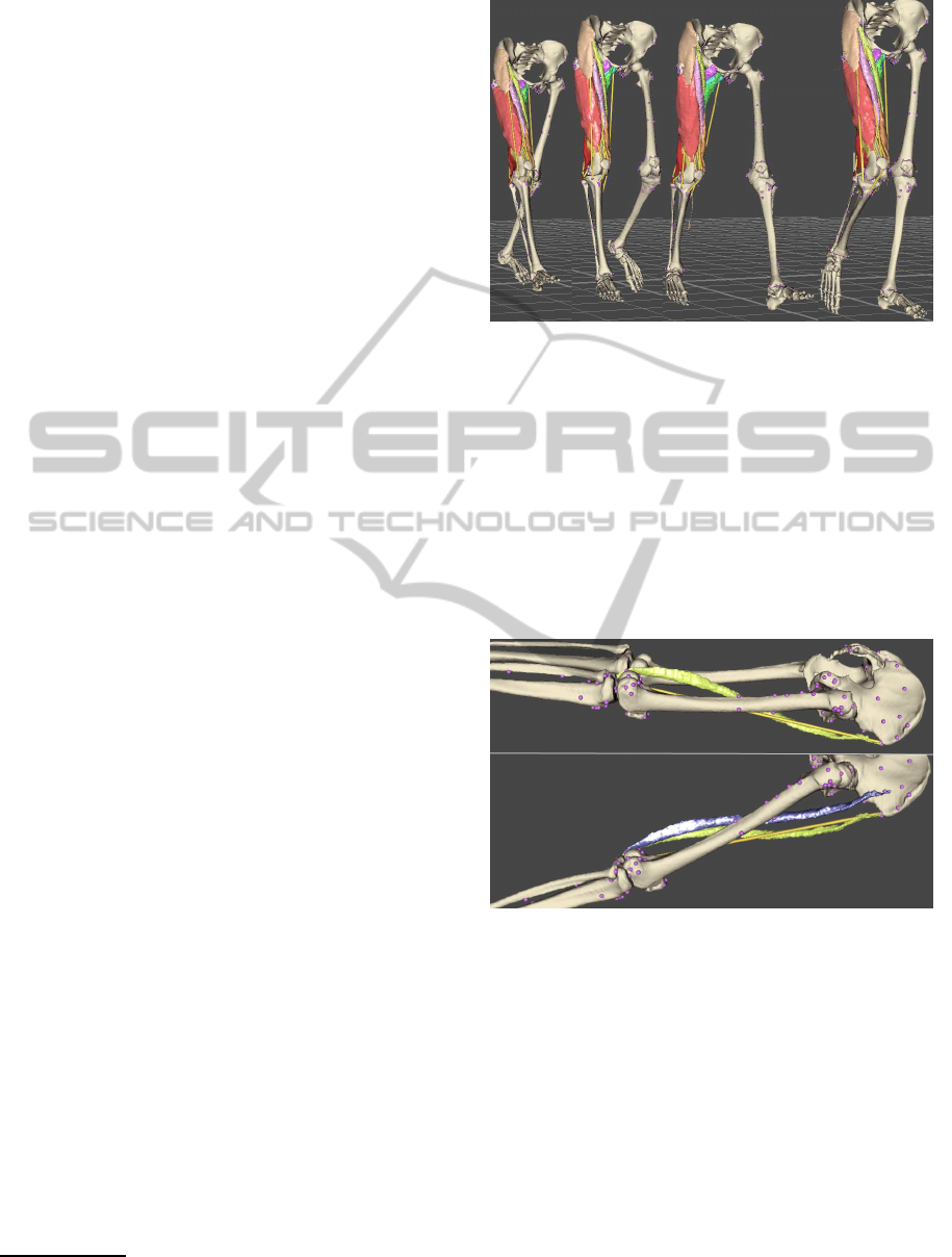
Figure 3 shows the deformation of muscles of

right thigh at current-pose frames t = 0.00, 0.25, 0.50

and 0.75 of the 1.56 seconds long walk sequence.

The deformation process of a single muscle con-

sumed 250–650 ms per frame on Intel Core i7 2.67

GHz computer, which makes the new method to be

about 8–20 times slower than our former deforma-

tion method that was based on the mesh skinning with

volume correction in post-processing (Kohout et al.,

2011). Nonetheless, the proposed method is still fast

enough for our purpose since the deformation of all

these muscles required a few seconds. We note that

this time does not include the time consumed in the

pre-processing to compute the coarse mesh and to es-

tablish the relationship between the both meshes (our

implementation takes up to one minute depending on

the model complexity).

http://graphics.zcu.cz/Projects/Muskuloskeletal-

Modeling

Figure 3: Wrapping of the muscles of right thigh during the

movement.

The shapes of the deformed and rigidly trans-

formed sartorius muscle are compared in Figure 4.

While the rigid transformation does not preserve the

attachment of the muscle to the bones and provides

the user with an unnatural result, the deformation pro-

duces a plausible result. The loss in the volume of the

muscle was about 0.02%, which is much lower than

the loss 11% observable in our former method.

Figure 4: Sartorius muscle with its action line (yellow) in

the rest-pose position (above) and at frame t = 0.00 of the

walk sequence (below), transformed rigidly (blue) and de-

formed (green) according to the change of its action line.

As it can be seen in Figure 5, the new method pre-

serves the volume much better also for other muscles

and other poses. Nevertheless, for some poses, the

maximal change in the volume of muscle may ex-

ceed 6%, which is, according to (Aubel and Thal-

mann, 2000)), the physiologically acceptable limit.

The reason for such a poor result is that the iterative

process terminated for semitendinosus muscle not be-

cause the optimal solution had been reached but be-

cause the maximal allowed number of iterations (100

in our case) had been performed. For all other mus-

GRAPP 2012 - International Conference on Computer Graphics Theory and Applications

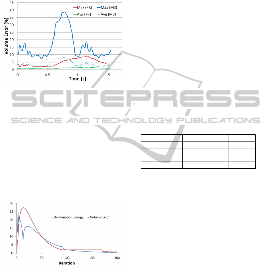
cles, the maximal volume error is within the physio-

logically acceptable limits.

Figure 5: Comparison of maximal and average volume er-

rors for muscles of the right thigh in the walk sequence for

our former method (M3) and the proposed one (PK).

The results can be easily improved by increas-

ing the maximal allowed number of iterations as it

is demonstrated in Figure 6 that shows the depen-

dence of the deformation energy and volume error

on the number of iterations for semitendinosus mus-

cle. More than 170 iterations were needed before

the deformation energy dropped to the level when the

method could start using the detailed mesh for the vol-

ume computation – see the abrupt change in the vol-

ume error function. Whilst the volume error was al-

most 10% after 100 iterations (see Figure 5), the ﬁnal

volume error (after 200 iterations) is about 0.04%.

Figure 6: Monotonic functions of the deformation energy

and the volume error in the dependence on the number of

iterations.

There are two main factors contributing to such

a slow convergence of the method. First, it has

been found that many tested muscles (semitendinosus

muscle included), extracted from MRI images during

our previous EU-funded project (LHDL, IST-2004-

026932) as described in (Testi et al., 2010), are not

closed manifolds. This causes troubles when creat-

ing the coarse mesh and expressing the relations be-

tween both meshes, which lead into an appearance of

ill-shaped triangles in the coarse mesh, and, if non-

manifold edges are present at a very narrow place

(typically, tendon part), also into having more than

just one component of the coarse mesh. As a re-

sult, the method needs more iterations and, further-

more, strange spikes on the deformed mesh may ap-

pear. This could be solved by reﬁning the muscles,

however, this is a part of our future work.

Next, for some muscles (e.g., sartorius), there is

only a loose relation between the muscle surface and

its skeleton, which negatively inﬂuences the number

of iterations required. This is demonstrated in Table 2

that shows the processing time needed for various

– already reﬁned – muscles of different sizes. Vas-

tus lateralis, which contains more than 50K triangles

but have skeleton going through its volume, was de-

formed faster than sartorius, which has less than 10K

triangles but its skeleton lies outside the mesh.

Table 2: Performance of our method on Intel Core i7 2.67

GHz, 12 GB DDR3 1.3GHz RAM.

Muscle Num. of Triangles Time [ms]

Rectus femoris 5238 268

Sartorius 9908 476

Adductor longus 13912 550

Vastus lateralis 50240 379

To reduce the required processing time, we par-

allelized routines for the multiplication of matrices,

the calculation of MVC coordinates of the muscle

mesh in the coarse mesh and the reconstruction of the

muscle mesh from the coarse one using OpenMP, a

multiplatform interface for parallel programming in

C, C++ and Fortran described, e.g., in (Gatlin and

Isensee, 2010). OpenMP allows automatic assign-

ment of independent iterations of a for cycle to work-

ing threads, providing that the cycle is preﬁxed in the

code by special directives as it is shown in Figure 7.

Table 3 shows the results of the parallelization.

The optimal performance obviously is achieved when

the number of threads to be used for the calculation

equals the number of physical cores of CPU. As it

can be seen, speed-up of at least 40% can be reached

on commodity hardware.

We have investigated also an option of speeding

up multiplication of matrices by employing GPU us-

ing CUBLAS library, which is a standard part of

CUDA system (nVidia, 2011). Providing that matri-

ces to be multiplied are represented by one dimen-

sional arrays, the speed-up on a system with NVIDIA

GeForce 9600 GT 512 MB is about 978, otherwise,

FAST DEFORMATION FOR MODELLING OF MUSCULOSKELETAL SYSTEM

Figure 7: Parallelization of the multiplication of matrices A

and B by OpenMP directives).

Table 3: Time needed by parallel version for processing a

mesh of 6978 vertices on Intel Core i7 4.4 Ghz.

Threads Time [ms] Speed-up

1 397 –

2 278 1.43

4 248 1.60

8 262 1.51

16 295 1.35

which is our case, it is only 2.26 because of the re-

quired transformation from the internal data structure

into the array and vice versa. Still this is an important

speed-up.

7 CONCLUSIONS

In this paper we described a gradient domain volume

preserving deformation method suitable for muscle

wrapping application. The deformation is governed

by the change of the action line (skeleton) of the mus-

cle mesh - the method iteratively alters the positions

of mesh vertices to adapt the change of the skele-

ton whilst preserving the volume. For any of tested

muscles, 200 iterations are enough to achieve vol-

ume error below 0.04%, 100 iterations are sufﬁcient

for any manifold muscles. The sequential process-

ing of typical mesh requires about 400 ms on com-

modity hardware. When parallelized using OpenMP

the required time may drop to 250 ms depending on

hardware conﬁguration and even to a couple of ms

(estimated) when parallelized using CUDA. Hence,

the method is fast enough to be used for the mus-

cle wrapping for clinical practise. An understandable

drawback of the approach is its sensitivity to the mesh

quality. For non-manifold meshes, which often result

from marching cube iso-surface extraction, the con-

vergence of the method may be very slow or even the

method may produce a mesh having some parts un-

naturally deformed (e.g., spikes appearance, strange

twists). Some mesh ﬁltering prior to the deformation

is, therefore, typically needed. This ﬁltering is a part

of our future work as well as proper validation of our

method in clinical context.

ACKNOWLEDGEMENTS

This work was supported by the Information Soci-

ety Technologies Programme of the European Com-

mission under the project VPHOP (FP7-ICT-223865).

The authors would like to thank the various people

who contributed to the realisation of the MAF and

LHPBuilder software and to various people who pro-

vided condition under which the work could be done.

REFERENCES

AnyBody (2010). Anybody technology,

http://www.anybodytech.com.

Arnold, A. S., Salinas, S., Asakawa, D. J., and Delp, S. L.

(2000). Accuracy of muscle moment arms estimated

from mri-based musculoskeletal models of the lower

extremity. Computer aided surgery ofﬁcial journal of

the International Society for Computer Aided Surgery,

5(2):108–119.

Aubel, A. and Thalmann, D. (2000). Efﬁcient muscle shape

deformation. In IFIP, pages 132–142.

Audenaert, A. and Audenaert, E. (2008). Global opti-

mization method for combined spherical-cylindrical

wrapping in musculoskeletal upper limb modelling.

Computer Methods and Programs in Biomedicine,

92(1):8–19.

Blanco, F. R. and Oliveira, M. M. (2008). Instant mesh de-

formation. Proceedings of the 2008 symposium on In-

teractive 3D graphics and games SI3D 08, 1(212):71–

78.

Blemker, S. S. and Delp, S. L. (2005). Three-dimensional

representation of complex muscle architectures and

geometries. Annals of Biomedical Engineering,

33(5):661–673.

Botsch, M. and Kobbelt, L. (2003). Multiresolution surface

representation based on displacement volumes. Com-

puter Graphics Forum, 22(3):483–491.

Debunne, G., Desbrun, M., Cani, M.-P., and Barr, A. H.

(2001). Dynamic real-time deformations using space

& time adaptive sampling. In Proceedings of the 28th

annual conference on Computer graphics and interac-

tive techniques, SIGGRAPH ’01, pages 31–36, New

York, NY, USA. ACM.

Delp, S. L. and Loan, J. P. (2000). A computational frame-

work for simulating and analyzing human and animal

movement. Computing in Science and Engineering,

2(5):46–55.

Erdemir, A., McLean, S., Herzog, W., and Van Den Bogert,

A. J. (2007). Model-based estimation of muscle forces

GRAPP 2012 - International Conference on Computer Graphics Theory and Applications

exerted during movements. Clinical Biomechanics,

22(2):131–154.

Favre, P., Gerber, C., and Snedeker, J. G. (2010). Auto-

mated muscle wrapping using ﬁnite element contact

detection. Journal of Biomechanics, 43(10):1931–

1940.

Gao, F., Damsgaard, M., Rasmussen, J., and Christensen,

S. T. (2002). Computational method for muscle-path

representation in musculoskeletal models. Biological

Cybernetics, 87(3):199–210.

Garner, B. and Pandy, M. (2000). The obstacle-set method

for representing muscle paths in musculoskeletal

models. Computer Methods in Biomechanics and

Biomedical Engineering, 3(1):1–30.

Gatlin, K. S. and Isensee, P. (2010). Reap

the beneﬁts of multithreading without all

the work. http://msdn.microsoft.com/en-

us/magazine/cc163717.aspx.

Hoppe, H. (1999). New quadric metric for simplifying

meshes with appearance attributes. Proc IEEE Con-

ference on Visualization VIS99, pages 59–66.

Huang, J., Shi, X., Liu, X., Zhou, K., Wei, L.-Y., Teng,

S.-H., Bao, H., Guo, B., and Shum, H.-Y. (2006).

Subspace gradient domain mesh deformation. ACM

Transactions on Graphics, 25(3):1126–1134.

Jensen, R. and Davy, D. (1975). An investigation of muscle

lines of action about the hip: A centroid line approach

vs the straight line approach. Journal of Biomechan-

ics, 8(2):103–110.

Ju, T., Schaefer, S., and Warren, J. (2005). Mean value

coordinates for closed triangular meshes. ACM Trans-

actions on Graphics, 24(3):561–566.

Kohout, J., Clapworthy, G. J., Martelli, S., Wei, H., Vice-

conti, M., and Agrawal, A. (2011). Fast muscle wrap-

ping. Computers & Graphics. Submitted for publica-

tion.

Li, S. Z. (1994). Markov random ﬁeld models in com-

puter vision. In Eklundh, J.-O., editor, ECCV (2), vol-

ume 801 of Lecture Notes in Computer Science, pages

361–370. Springer.

Marsden, S. P. and Swailes, D. C. (2008). A novel approach

to the prediction of musculotendon paths. Proceed-

ings of the Institution of Mechanical Engineers Part H

Journal of engineering in medicine, 222(1):51–61.

Nealen, A., Igarashi, T., Sorkine, O., and Alexa, M. (2006).

Laplacian mesh optimization. In Proceedings of the

4th international conference on Computer graphics

and interactive techniques in Australasia and South-

east Asia, GRAPHITE ’06, pages 381–389, New

York, NY, USA. ACM.

nVidia (2011). Cuda zone. http://developer.nvidia.com/ca

tegory/zone/cuda-zone.

OpenSim (2010). Opensim project, https://simtk.org/home

/opensim.

Rohmer, D., Hahmann, S., and Cani, M.-P. (2008). Lo-

cal volume preservation for skinned characters. Com-

puter, 27(7):1919–1927.

Schroeder, W., Martin, K., and Lorensen, B. (2004). The

Visualization Toolkit, Third Edition. Kitware Inc.

Testi, D., Quadrani, P., and Viceconti, M. (2010). Phys-

iomespace: digital library service for biomedical

data. Philos Transact A Math Phys Eng Sci,

368(1921):2853–2861.

van der Helm, F. and Veenbaas, R. (1991). Modelling the

mechanical effect of muscles with large attachment

sites: Application to the shoulder mechanism. Journal

of Biomechanics, 24(12):1151–1163.

Viceconti, M., Astolﬁ, L., Leardini, A., Imboden, S.,

Petrone, M., Quadrani, P., Taddei, F., Testi, D., and

Zannoni, C. (2004). The multimod application frame-

work. Information Visualisation, International Con-

ference on, 0:15–20.

Von Funck, W., Theisel, H., and Seidel, H. P. (2008).

Volume-preserving mesh skinning. In Vision Model-

ing and Visualization, pages 409–414. IOS Press.

VPHOP (2010). the osteoporotic virtual physiological hu-

man, http://vphop.eu.

Xu, W.-W. and Zhou, K. (2009). Gradient domain mesh

deformation a survey. Journal of Computer Science

and Technology, 24(1):6–18.

Zhou, K., Huang, J., Snyder, J., Liu, X., Bao, H., Guo, B.,

and Shum, H.-Y. (2005). Large mesh deformation us-

ing the volumetric graph laplacian. ACM SIGGRAPH

2005 Papers on SIGGRAPH 05, 1(212):496.

FAST DEFORMATION FOR MODELLING OF MUSCULOSKELETAL SYSTEM