
HEAD SHAPE ESTIMATION USING A PARTICLE FILTER
INCLUDING UNKNOWN STATIC PARAMETERS
Catherine Herold
1,2,3,4
, Vincent Despiegel
1,2
, St´ephane Gentric
1,2
,
S´everine Dubuisson
4
and Isabelle Bloch
1,3
1
Identity & Security Alliance (The Morpho and T´el´ecom ParisTech Research Center), Paris, France
2
Morpho, Safran Group, 11 boulevard Galli´eni, Issy-les-Moulineaux, France
3
T´el´ecom ParisTech, CNRS LTCI, Paris, France
4
LIP6, Universit´e Pierre et Marie Curie, 4 place Jussieu, Paris, France
Keywords:
Particle Filter, Shape Parameter Estimation, 3D Morphable Model.
Abstract:
We present a particle filter algorithm to optimize the static shape parameters of a given face observed under
multiple views and during time. Our goal is to determine the 3D shape of the head given these observations, by
selecting the most suitable deformation parameters. The main idea of our method is to integrate the unknown
static parameters in the particle filter hidden state and to filter and modify these parameter values given the
recursively incoming observations. We propose here a comparative study of different variants of this approach
evaluated on synthetic data. These results show the potential given by this type of particle based methods,
which have mainly been presented from a theoretical point of view until now. We conclude with a discussion
on the adaptation of these methods to real data sequences.
1 INTRODUCTION
Recent improvements in face matching algorithms
have led to an increased interest in facial biome-
try. Nevertheless, for most of these algorithms, a
valid frontal view of the head is required to compute
the matching score with a frontal reference picture.
For Video-Based Face Recognition, obtaining such
frontal views is still an issue, especially when the ac-
quisition process has to be fast in an unconstrained
scenario. A classical configuration would be a set of
cameras situated around a door, acquiring videos of
the people passing through to authenticate them “on
the fly”. Due to the camera setup and to the “on the
fly” scenario, there is no guarantee to have a frontal
view directly in any of the input images.
An intermediate step is then required before the
matching step, which consists in estimating the pose
of the head in each view, extracting its characteristics
and recovering a frontal view from the observations.
This is usually done by using a three-dimensional
head model, which is fitted to the observations by op-
timizing different parameters (pose, shape, texture).
Given this individualized model, it is then possible to
synthesize views of the head under any pose. Among
all existing head models, the 3D Morphable Model
(3DMM) introduced in (Blanz and Vetter, 1999) has
been widely used in the last decade. Most of the al-
gorithms used to fit this 3D head model are based
on iterative methods, like Levenberg-Marquardt op-
timization (Romdhani and Vetter, 2005), to minimize
a cost function composed of one or several criteria.
The main drawback using these methods is their sen-
sitivity to the initialization. Depending on the starting
hypothesis, a local minimum can be obtained, which
can be far away from the global optimum in case
of outliers or noisy observations. As the matching
score depends on the quality of the head estimation,
it is worthwhile to use all the available observations
in the sequence to accurately determine the shape.
To our knowledge, only few works have been done
on temporal fusion to estimate facial shape parame-
ters. One proposal has been made by (Van Rootseler
et al., 2011) and consists in computing the mean of
the shape parameters over a set of estimations associ-
ated to each timestamp. However, each estimation is
done independently at each time, without using previ-
ous information.
In order to deal with the problem of local minima
and to account for the temporal information, we pro-
pose an alternative method to evaluate the best shape
parameters: we use a particle filter method which can
284
Herold C., Despiegel V., Gentric S., Dubuisson S. and Bloch I..
HEAD SHAPE ESTIMATION USING A PARTICLE FILTER INCLUDING UNKNOWN STATIC PARAMETERS.
DOI: 10.5220/0003855002840293
In Proceedings of the International Conference on Computer Vision Theory and Applications (VISAPP-2012), pages 284-293
ISBN: 978-989-8565-04-4
Copyright
c
2012 SCITEPRESS (Science and Technology Publications, Lda.)
take unknown hidden parameters (the shape) into ac-
count. The Bayesian context allows for a recursive
update of the shape parameter estimation, instead of
making independent hypotheses at each frame. Al-
though such methods have already been presented
from a theoretical point of view and illustrated with
scholar examples (Storvik, 2002; Fearnhead, 2002;
Andrieu et al., 2005), only few works have been done
in computer vision applications.
After presenting the context of our work and some
details on the head model in Section 2, we recall the
use of particle filter for dynamic state filtering in Sec-
tion 3. The extension to methods dealing with static
unknown parameters is given in Section 4. We then
propose an adaptation of one of them to the temporal
head shape estimation issue, which is the main contri-
bution of this paper. As another contribution, in Sec-
tion 5, we present comparative results of some varia-
tions of this method, using a synthetic databasefor the
evaluation. Given the encouraging results with parti-
cle filter methods, we conclude this article by men-
tioning the extension to real data in Section 6.
2 CONTEXT AND HEAD MODEL
2.1 On the Fly Authentication
The final aim of our application is to authenticate
a person walking through a gate or a corridor in
an unconstrained scenario. To this aim, we bene-
fit from video streams acquired by a set of cameras
situated around the outdoor and directed toward the
corridor area. As the faces are observed under non
frontal poses, our goal is to compute the correspond-
ing frontal view given the images. Using several im-
ages can improve the accuracy of the head recon-
struction; indeed, while people are getting close to
the cameras, the head is seen under new poses, and
some new parts of the head appear. These are useful
to complete the previously estimated model and elim-
inate wrong hypotheses. This is why we propose a
method based on the whole stream in this article.
2.2 Head Model
As underlined before, our final aim is to estimate as
accurately as possible the shape and texture of the ob-
served head to validate the authentication. We em-
ploy a 3D head model based on the 3DMM intro-
duced by (Blanz and Vetter, 1999). In this paper, we
focus on the geometrical part (shape) of the model.
This shape model is constructed from a set of M 3D
face scans, for which a full correspondence has been
computed (meaning that each 3D vertex X
v
model
of a
generic model has been associated to the correspond-
ing position X
v
for each face). The set of 3D vertices
of one head forms a mesh characterizing the shape.
The mean shape
¯
S and the main deformation axes
{s
i
,i ∈ 1 : M− 1} are then computed by a Principal
Component Analysis (PCA). Each shape of the space
can finally be written as:
S =
¯
S+
M− 1
∑
i=1
θ
i
s
i
(1)
where the shape vector θ = (θ
1
,...,θ
M− 1
) is dis-
tributed with the following probability:
p(θ) ∼ e
−
1
2
∑
M−1
i=1
(
θ
i
σ
i
)
2
(2)
with σ
2
i
,i
th
eigenvalue of the shape covariance matrix
(see (Blanz and Vetter, 1999) for more details).
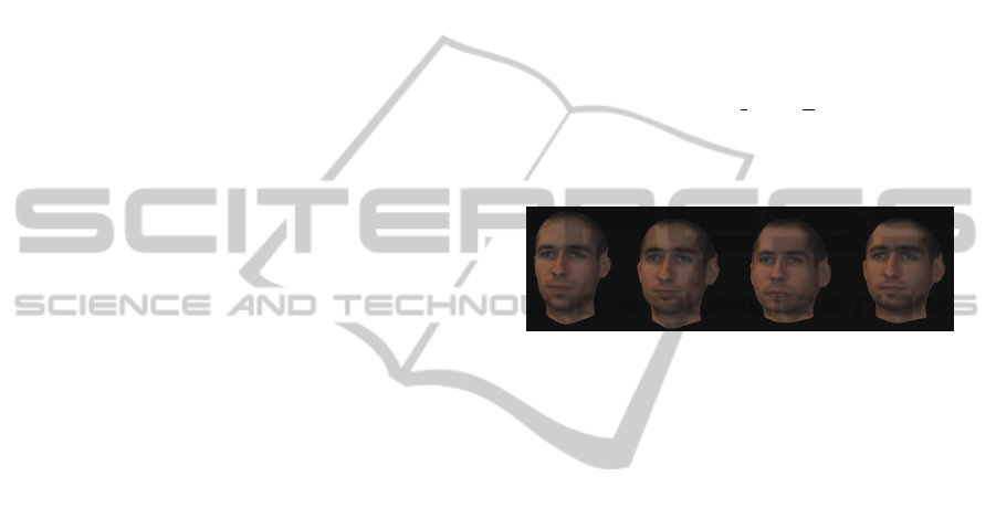
Figure 1: Some samples of head appearance for different
sets of shape parameters (and a common texture map).
Figure 1 shows some instances created from this
3D shape model, using a fixed texture map. This para-
metric head shape model has two main advantages.
First, the number of unknownparameters determining
the shape is widely reduced thanksto PCA. Moreover,
by characterizing a face as a linear combination of
eigenvectors, we take naturally into account the prior
given by the learning database to regularize the solu-
tion.
3 PARTICLE FILTER FOR
DYNAMIC STATE ESTIMATION
We briefly introduce particle filter methods for dy-
namic state tracking. A complete overview can be
found in (Doucet et al., 2000). Let x
t
be the (time-
varying) hidden state to estimate, and y
t
an observa-
tion. In our case, x
t
corresponds to the 3D head pose
at time t and y
t
to the set of available views at this
time. We make the assumption that (x
t
)
t=0,...,T
is a
Markov process, meaning that x
t
only depends on the
previous state x
t−1
. These two states are linked by
the prediction equation, x
t
= f(x
t−1
,η
t
), where f is
the transition function and η
t
is the noise related to
the state dynamics. The observations are linked to the
current state by the measurement function g and an
associated measurement noise γ
t
: y
t
= g(x
t
,γ
t
).
HEAD SHAPE ESTIMATION USING A PARTICLE FILTER INCLUDING UNKNOWN STATIC PARAMETERS
285

Tracking processes are often expressed in a
Bayesian framework (Isard and Blake, 1998). In this
context, the aim is to estimate the density of the cur-
rent state given all previous and current observations,
written p(x
t
|y
0:t
). This probability is computed in a
recursive way, and given by:
p(x
t
|y
0:t
) ∝ p(y
t
|x
t
)
| {z }
likelihood
Z
X
state dynamics
z }| {
p(x
t
|x
t−1
) p(x
t−1
|y
0:t−1
)
| {z }
previous density
dx
t−1
,
(3)
where X is the dynamic state space.
When the transition and the measurement func-
tions are linear, and η
t
and γ
t
are Gaussian addi-
tive noises, the probability can be computed in an
analytical way with the Kalman filter. To handle
other cases, particle filters have been proposed in the
1990’s. In this context, the posterior p(x
t
|y
0:t
) is esti-
mated by a sequential Monte-Carlo method with a set
of N weighted particles. Each particle x
(i)
t
represents
a possible realization of the state x
t
, and its weight
w
(i)
t
evaluates its consistency given the observations.
The probability p(x
t
|y
0:t
) is then approximated by
p(x
t
|y
0:t
) ≈
∑
N
i=1
w
(i)
t
δ(x
(i)
t
−x
t
). Given the initial par-
ticles set
n
(x
(i)
0
,w
(i)
0
),i = 1 : N
o
, the posterior density
is recursively estimated at each timestamp using three
steps. First, during the prediction step, each particle
x
(i)
t−1
moves from time t − 1 to time t given the prob-
ability p(x
t
|x
t−1
) associated with the system dynam-
ics. The weights w
(i)
t
are then updated according to
the current observation y
t
, using p(y
t
|x
(i)
t
). Finally, a
resampling is performedif the particle weights are too
spread.
The particle filter outcome depends on the num-
ber of particles used to approximate the density over
the hidden state space. Indeed, if too few particles are
sampled in the space, the subregions containing the
most probable parameters are not necessarily visited,
and the filter remains uninformative. When increas-
ing the size of the particle state space by including
new parameters, it is therefore necessary to adapt the
number of particles.
4 PARTICLE FILTER WITH
UNKNOWN PARAMETERS
At this stage, we can point out that the head shape
(which is unknown at the beginning of the sequence)
influences the pose evaluation. Indeed, if we estimate
the pose of a distorted head using the mean shape
model, a perfect fitting will probably not be possible,
and the shape difference will be balanced by a pose
correction. For instance, for someone having a thin
head, ears are close to the eyes, which is not the case
for the mean model used for the pose estimation. The
yaw angle may then be overestimated to reduce the
distance between the ear and the eye projections.
Moreover, for biometric applications, we are not
only interested in these pose parameters at each time,
but also in the shape parameters explaining the whole
set of observations, in order to associate the correct
pixel with each 3D vertex, and generate an accurate
frontal view at the end of the process. This issue
is the subject of this section, presenting a short re-
view of particle filter algorithms when unknown static
parameters have to be taken into account and esti-
mated. We especially develop how these methods can
be adapted to estimate the unknown head shape pa-
rameters, given a set of observations acquired recur-
sively in time.
4.1 Particle Filter for Static Parameter
Estimation
Let θ be the vector of dimension s
θ
containing all un-
known static shape parameters, and Θ the associated
parameter space. We can rewrite the particle filter
equations when θ has to be taken into account (and
eventually evaluated):
x
t
= f(x
t−1
,η
t
)
y
t
= g(x
t
,θ,γ
t
) = g
θ
(x
t
,γ
t
)
(4)
where x
t
is the time-varying head pose (i.e. the 3D
head center position and the head orientation). θ does
not appear in the first equation as the head shape does
not influence the pose dynamics. However, the sec-
ond equation depends on θ, as the shape parameters
modify each 3D head vertex position, and therefore
its associated projection in the images.
In order to account for the presence of unknown
parameters, several methods have already been ex-
plored, mostly theoretically. In (Kantas et al., 2009),
the authors list a set of existing methods to estimate
static parameters using particle filters. One can sepa-
rate the offline methods, which use simultaneously all
the observations to make a unique global optimiza-
tion, from online methods, which update recursively
the parameter estimation when new observations be-
come available. We consider only this second case,
adapted to our application, where each observation
(y
t
,t = 1, ..., T) corresponds to a frame of a video
stream. The aim is to recursively compute an esti-
mation θ
∗
each time a new observation is available.
Among online approaches, particle filter methods
with unknown static parameters can proceed in two
different ways:
VISAPP 2012 - International Conference on Computer Vision Theory and Applications
286

1. compute an estimation θ
∗
by expectation-
maximization or gradient descent methods. The
optimization returns directly a unique value for
θ
∗
. This method aims at maximizing the marginal
likelihood p
θ
(y
1:t
), thanks to a deterministic or
stochastic gradient descent method:
θ
t
= θ
t−1
+ γ
t
∇
θ
log p
θ
1:t−1
(y
t
|y
1:t−1
) (5)
using Monte-Carlo techniques to approximate the
score ∇log p
θ
1:t−1
(y
t
|y
1:t−1
).
2. integrate the static parameters in the hidden state,
thus increasing the state dimension. Monte-Carlo
methods are then used to estimate the join den-
sity p(θ,x
1:t
|y
1:t
) over the mixed state, which can
be marginalized with respect to the dynamic state
x
1:t
. A specific value of θ
∗
can be obtained from
this approximated density, as the best particle
state or the mean over the particle set.
Due to the sensitivity to initialization of gradient
algorithms (Kantas et al., 2009), we favor the sec-
ond way of estimating θ
∗
, which integrates the static
parameters in the particle state. Nevertheless, some
types of artificial moves introducedin the coming part
may create a bias on the estimation accuracy.
4.2 Introducing Unknown Parameters
in the State Space
Several authors (Storvik, 2002; Fearnhead, 2002;
Minvielle et al., 2010) suggest to integrate the static
parameters in the particle state. The complete state
to evaluate becomes the concatenation ξ = { x,θ} ∈
X × Θ, where x is the head pose and θ the static
parameters (the shape weighting factors in Equation
(1)). Each particle will then represent both a shape
parameter hypothesis and an associated pose.
From the particle filter defined over the mixed
state, one can infer the distribution p(θ|y
1:t
) by in-
tegrating on the dynamic state space X
t
:
p(θ|y
1:t
) =
Z
X
t
p(x
1:t
,θ|y
1:t
)dx
1:t
. (6)
As underlined in several papers, the integration of
static parameters in the hidden state can lead to im-
poverishment issues if no dynamics are used in the
evolution process (although by definition, the static
parameters do not change with time). Indeed, due to
resampling steps, most of the initial values will grad-
ually disappear, leading to a restrictive set of possi-
ble values. Moreover, only the initially sampled pa-
rameters can be evaluated and selected. It is there-
fore required to include particle state moves between
two evaluations, despite their static aspect, in order to
allow a better shape space exploration. This can be
done with artificial and systematic dynamics, smart
diversification parametrized by the particle weights or
specific sampling procedures. We present the various
moves tested in our case.
Artificial Dynamics. As in (Minvielle et al., 2010),
we apply a fixed and automatic artificial dynamic on
the static parameters for all particles. Given a particle
(x
(i)
t−1
,θ
(i)
t−1
,w
(i)
t−1
), this artificial dynamic will lead to
the new shape parameters at time t:
θ
(i)
t
= θ
(i)
t−1
+ n
θ
, (7)
where n
θ
is a Gaussian noise with zero mean.
An intuitive idea is to use the particle weight to
adapt the noise applied on the static parameters. In-
deed, if a particle has a small weight, the current
parameters might be distant from the true ones, this
is why it is useful to strongly modify them in order
to explore another space area of the shape parame-
ters. Conversely, if the current weight is high, it is
interesting to look around the current state to search
for a possible higher value (local optimization). To
take this into account, we propose a modified version
of the previous artificial move algorithm by making
the noise n
θ
in Equation (7) dependent on the parti-
cle weight w
(i)
t−1
to improve the particle moves in the
static space. More specifically, the noise variance is
inversely proportional to the weight.
MCMC Moves. In (Fearnhead, 2002), the parti-
cle diversity in the static parameter space is obtained
thanks to a step of MCMC (Monte Carlo Markov
Chain) process. This step allows conditional particle
moves in subspaces with high probability, by adding
a Gaussian noise to the static state (this contrasts with
the resampling step, which keeps each sampled par-
ticle identical to the original one). This idea, called
Resample-Move algorithm, has been introduced in
(Gilks and Berzuini, 2001). The process is the follow-
ing: at each timestamp t, a MCMC move is generated
given a kernel K
t
(x
′
1:t
,θ
′
|x
1:t
,θ), having p(x
1:t
,θ|y
1:t
)
as invariant distribution. This move can be applied on
the static parameters θ only:
K
t
x
′
1:t
,θ
′
|x
1:t
,θ
= δ
x
1:t
x
′
1:t
p
θ
′
|y
1:t
,x
1:t
(8)
and can be obtained with a Gibbs sampler or with a
two-step Metropolis-Hastings (MH) algorithm:
1. Sample randomly a candidate θ
′
t
∼ p(θ
′
t
|θ
t
)
2. Sample v ∼ U
[0,1]
.
If v ≤ min
1,
p(y
1:t
|x
1:t
,θ
′
)
p(y
1:t
|x
1:t
,θ)
(9)
HEAD SHAPE ESTIMATION USING A PARTICLE FILTER INCLUDING UNKNOWN STATIC PARAMETERS
287

the move towards θ
′
is accepted; otherwise, θ is kept.
We can underlineherethat it can be costly to apply
this formula directly. Indeed, even if we only change
the static parameters, this modification requires to
keep in memory all previous observations and to re-
compute all the likelihood values at previous times,
which is computationally more and more expensive.
This is why we introduce a period ∆T, which char-
acterizes the number of frames used for the MCMC
validation. The move validation depends then on:
v ≤ min
1,
p(y
t−∆T:t
|x
t−∆T:t
,θ
′
)
p(y
t−∆T:t
|x
t−∆T:t
,θ)
, (10)
with ∆T = 0 if we only use the current observations.
The Bayesian method including a MCMC sam-
pling step has the advantage to keep the probability
p(θ|y
0:t
) invariant, unlike the basic method which in-
troduces a bias due to the Gaussian noise added on
static parameters. Nevertheless, these methods need
more evaluation steps (one more per particle during
the move validation), and are not robust when t ≫ 1.
As in our case, t is limited by the number of available
frames (about 20) and as we only have a few parame-
ters to estimate, we are in the conditions underlined in
(Kantas et al., 2009) for which this method is suitable.
As in the case of systematic Gaussian noise addi-
tion on the static parameters, the MH-sampling step
only allows a local diversification of the static pa-
rameters. Another option we propose is to make a
global sampling step from the current approximation
p(θ|y
0:n
) (or a prior on the static parameters), inde-
pendently of the particle current state (x
(i)
t
,θ
(i)
t
). Intu-
itively, this means that any move is allowed, as long
as the likelihood is improved with the new set of pa-
rameters. This helps the particles to get out from local
maxima when more likely states exist.
4.3 Likelihood Functions
When estimating the head shape parameters, there is
a specific difficulty due to the non-trivial relation be-
tween the unknown shape and pose on the one hand,
and the corresponding observation on the other hand.
The function g in Equation (4), which can be related
to the update step, contains actually the head model
deformation, its pose transformation, and finally the
projection function to obtain the images. Special at-
tention shouldbe paid to the likelihood functionsused
at this point.
We describe here more precisely the functions
used in the proposed algorithm for face shape esti-
mations. During the observation step, the particle
weights are updated according to the particle agree-
ment with the current observations, using three differ-
ent likelihood functions:
• one is derived froma distance between the 2D fea-
ture point inputs and their retroprojection in each
view given the particle pose and shape parameters
(Figure 2(a)).
• the second one is derived from the direction sim-
ilarity between the gradients of the internal edges
(Figure 2(b)) projected from the model, and the
observed gradients at the same image location.
• the third one is derived from the silhouette simi-
larity (Figure 2(c)) and is computed in the same
way as the internal edge score.
(a) Feature points (b) Internal edges (c) Silhouette
Figure 2: Features used for the likelihood computation.
Under independence hypotheses on the edge and
feature point detectors, the three probabilities derived
from these scores can be multiplied to obtain the
global likelihood. Algorithm 1 summarizes the global
process of parameter estimation.
Algorithm 1: Static shape parameter estimation with a par-
ticle filter.
Sample the shape parameters θ from a prior Gaus-
sian distribution to initialize the set of particles
{(x
(i)
0
,θ
(i)
0
,w
(i)
0
= 1/N),i = 1 : N}
for f = 1 → N
frames
do
Input: noisy 2D feature point positions.
Mean shape model fitting to estimate the initial
pose x
0
t
using the method by (Umeyama, 1991).
for i = 1 → N do
- Sample around the estimated pose:
x
(i)
t
= x
0
t
+ n
x
, with n
x
∼ N(0,Σ
x
). (11)
- (Optional) Samplearound the previousshape
parameters: θ
(i)
t
= θ
(i)
t−1
+ n
θ
, with n
θ
∼
N(0,Σ
θ
).
- Update the weight with the likelihood
p(y
t
|x
(i)
t
,θ
(i)
t
): w
(i)
t
∝ w
(i)
t−1
p(y
t
|x
(i)
t
,θ
(i)
t
).
end for
Resampling
for i = 1 → N do
(Optional) Apply a MCMC move
end for
end for
VISAPP 2012 - International Conference on Computer Vision Theory and Applications
288
5 RESULTS ON SIMULATED
DATA
5.1 Data Generation and Evaluation
To evaluate the different particle filter versions pre-
sented in Section 4.2 (systematic noise addition, pos-
sibly parametrized by the weight and MCMC with lo-
cal or global sampling), we concentrate our work on
synthetic data in order to benefit fromthe ground truth
values for the pose and the shape parameters.
The test faces are generated with two shape pa-
rameters (s
θ
= 2) sampled from the standard normal
law, the pose during the sequence is similar to the one
in real sequences, and the images are obtained with
the same calibration parameters as in our acquisition
system.
We applied the different particle filter methods on
noisy data (σ = 2 pixels for the feature point inputs),
to simulate detector answers on real data. This leads
to an approximate pose initialization and to a score
function disturbed by this noise. The proposed ex-
perimental analysis is novel and provides a deeper in-
sight on the different particle filter methods of Section
4 applied on face image sequences. It presents the
possibilities offered by particle methods, when com-
plex transformations are involved between the obser-
vations (the image sequences) and the hidden state
(pose and shape parameters).
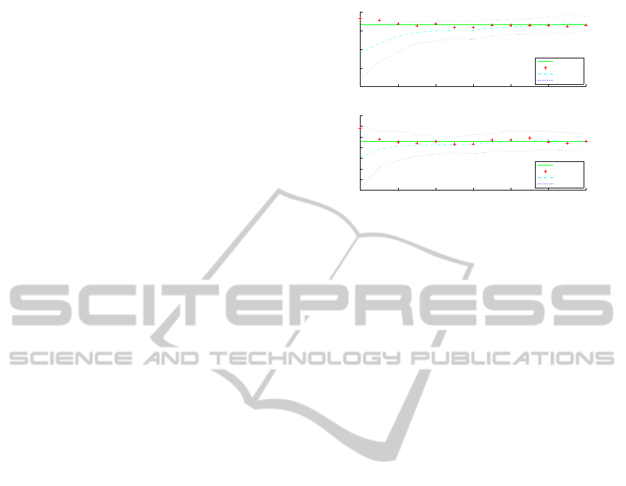
5.2 Parameter Convergence
5.2.1 With Known Dynamic State
In a first experiment, we check the convergence of
the particle static states towards the correct shape pa-
rameters when the head pose is known. In this case,
the only unknowns are the two static shape parame-
ters. The best particle and the filter mean and vari-
ance are plotted for one sequence in Figure 3. They
can be compared to the ground truth values plotted in
green solid line(GT). We can observethat the mean of
the filter converges towards the real parameters, and
that the variance decreases at the beginning of the se-
quence before stabilizing. In this example, even if
few particles are sampled around the true first param-
eter at the initialization step, the whole set of particles
moves towards this value over the sequence.
5.2.2 With Unknown Dynamic State
To simulate real data issues, in which the pose is not
known, we now integrate the hidden dynamic state x
t
in the estimation process. Besides the two unknown
0 2 4 6 8 10 12
−0.5
0
0.5
1
1.5
Frame
Parameter value
Coef 1
GT
best particle
mean
sigma
0 2 4 6 8 10 12
−0.2
0
0.2
0.4
0.6
0.8
1
1.2
Frame
Parameter value
Coef 2
GT
best particle
mean
sigma
Figure 3: Evolution of the filter static parameters when the
pose is known. 100 particles are used, artificial moves are
Gaussian noises with fixed covariance.
shape parameters already estimated before, there are
now six more time-varying unknowns, corresponding
to the 3D position and the 3 rotation angles. This ex-
plains why we use more particles in the coming ex-
periments, still conducted on synthetic data.
Robustness to the Pose Error. We initially evalu-
ate the algorithm robustness to an initial pose error.
To this aim, we launch the algorithm using various
input poses as initial pose estimation x
0
t
in Equation
(11): first the true pose, before adding various yaw
angle errors (2, 4, 6, 8 and 10 degrees). Particle
poses are then sampled around this modified pose in-
put. Figure 4 illustrates the results for these replays,
and shows that below 8 degree error on the initial
yaw estimation, the convergence results are compa-
rable. For higher errors, too few particles are sampled
around the true pose which makes the convergence
less probable. An higher dynamic noise n
x
in Equa-
tion (11), associated with more particles can be con-
sidered if larger pose errorsare expected. However, in
our study, the initial pose remains generally below the
convergence threshold. Further study on robustness
to simultaneous position and angle errors will help to
optimize these two parameters.
In fact, the true pose is not available, the pose is
therefore initialized as follows for the rest of the eval-
uation: the input feature point detections are used to
fit the mean model, and the resulting pose x
0
t
is used
to initialize the particle dynamic states (Algorithm 1).
Gaussian Noise on the Static Parameters. Figure
5 shows the filter evolution for the same sequence as
in Figure 3, but with unknown pose parameters. The
artificial dynamic is a Gaussian noise with fixed co-
variance for all particles. We can observe that the de-
viation is larger than in the previous case. As the pose
has to be estimated simultaneously, the particles hav-
HEAD SHAPE ESTIMATION USING A PARTICLE FILTER INCLUDING UNKNOWN STATIC PARAMETERS
289
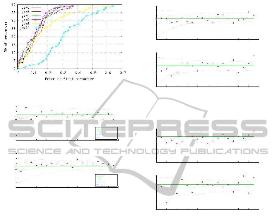
Figure 4: Robustness to the initial yaw angle error. From 0
degree (yaw0) to 10 (yaw10).
0 2 4 6 8 10 12 14 16 18 20
−1.5
−1
−0.5
0
0.5
1
1.5
2
Frame
Parameter value
Coef 1
GT
best particle
mean
sigma
0 2 4 6 8 10 12 14 16 18 20
−1.5
−1
−0.5
0
0.5
1
1.5
2
Frame
Parameter value
Coef 2
GT
best particle
mean
sigma
Figure 5: Evolution of the filter static parameters when the
pose is unknown. 2500 particles, artificial moves are Gaus-
sian noises with fixed covariance.
ing correct poses but wrong shape parameters might
be weighted as the ones having the inverse configu-
ration. The shape parameter filtering takes therefore
more time to converge.
Adaptive Noise. Figure 6 shows some convergence
results with 2500 particles, given input data without
noise.
Adding a noise of 2 pixels on the feature point po-
sitions, we get the results presented in Figure 7. De-
spite this observation alteration, the filter means for
the static parameters are close to the true values.
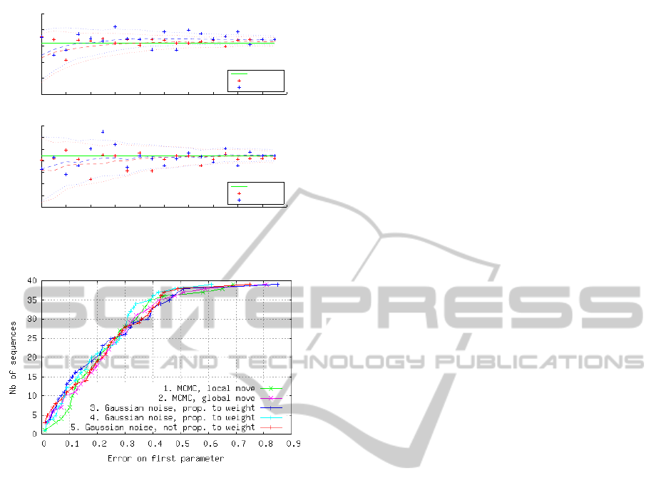
MCMC Moves. this method uses a validation step
before modifying the static parameters sampled for a
particle. We evaluate two types of sampling: local
sampling around the current value, and global sam-
pling given the Gaussian prior. The move is only ap-
plied on the static shape parameters, thus optimizing
the shape at a fixed pose. This step implies a new
likelihood computation, that should theoretically be
done on the whole set of observations y
0
,...,y
t
. In
this case, the validity of the pose x
(i)
0
,...,x
(i)
t−1
is ques-
0 2 4 6 8 10 12 14 16 18 20
−1
−0.5
0
0.5
1
1.5
2
2.5
Frame
Parameter value
Coef 1
0 2 4 6 8 10 12 14 16 18 20
−1.5
−1
−0.5
0
0.5
1
1.5
2
Frame
Parameter value
Coef 2
Figure 6: Evolution of the filter static parameters, when the
pose is unknown. No noise is added on the input feature
points. Artificial moves are Gaussian noises with adaptive
covariance.
0 2 4 6 8 10 12 14 16 18 20
−1.5
−1
−0.5
0
0.5
1
1.5
2
Frame
Parameter value
Coef 1
0 2 4 6 8 10 12 14 16 18 20
−1.5
−1
−0.5
0
0.5
1
1.5
Frame
Parameter value
Coef 2
Figure 7: Evolution of the filter static parameters when the
pose is unknown. Noise is added on the input feature points.
2500 particles, artificial moves are Gaussian noises with
adaptive covariance.
tionable and may be wrong. By using these pose pa-
rameters, the shape values which have been validated
with these poses will be preferred. This is why we use
∆
T
= 0, meaning that only the current view is used to
compute the move acceptation. Figure 8 shows the fil-
ter evolution for the two types of sampling methods,
which lead to similar results.
Methods Comparison. Let θ
1
GT
be the true value of
the first shape parameter and θ
1
eval
the meanvalue over
the particle states. To evaluate the different methods,
we measure the error ε = |θ
1
eval
− θ
1
GT
| for our 39 syn-
thetic sequences on the last frame of the sequence.
Figure 9 shows that all methods provide globally sim-
ilar results.
Curves 3, 4 and 5 present results when a system-
atic noise is added at each time on the static param-
eters. Using an adaptive noise (curve 4) instead of a
VISAPP 2012 - International Conference on Computer Vision Theory and Applications
290
0 2 4 6 8 10 12 14 16 18 20
−2
−1
0
1
2
3
Frame
Parameter value
Coef 1
GT
MCMC local
MCMC global
0 2 4 6 8 10 12 14 16 18 20
−1.5
−1
−0.5
0
0.5
1
1.5
2
Frame
Parameter value
Coef 2
GT
MCMC local
MCMC global
Figure 8: Evolution of the filter static parameters when the
pose is unknown. 2500 particles, MCMC moves.
Figure 9: Cumulative error distribution. The prior on θ is
(m = 0,σ = 1.7) for curves 1, 2, 4, 5 and (m = 0, σ = 1.0)
for curve 3.
fixed noise (curve 5) results in more accuracy thanks
to a better state space exploration. We can also notice
that the prior sampling on the parameter space (nor-
mal law with parameters (m = 0,σ = 1.0) for curve
3, (m = 0,σ = 1.7) for curve 4) influences slightly
the curves: with a wide distribution, it becomes easier
to reach large values of the parameters, as more parti-
cles will then be sampled around the true value. Con-
versely, for narrow initial sampling, the particles are
concentrated in a smaller area, which leads to more
accurate results when the parametersare close to zero.
This explains why curve 3 is above the others for
small errors. The highest error is around 0.6 for the
wide sampling (curve 4), against 0.85 using standard
normal law (curve 5). These values can be compared
to the interval covered by all θ
1
GT
of our database,
[−2.97;2.10], sampled from the standard normal law.
Using the weight adaptive noise method and a large
deviation for the initial parameter sampling, 87% of
replays verify ε ≤ 0.34 (6.7% of the interval width).
Although MCMC moves involve a validation step
using the Metropolis-Hastings algorithm, the two
evaluated methods (curves 1 and 2) do not outper-
form the previous ones, based on a systematic noise
addition. Automatic noise methods may therefore be
preferred since the other methods do not provide sig-
nificant accuracy improvements despite their higher
computational cost.
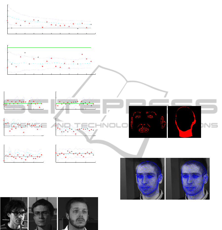
Failure Cases. For some sequences, the true values
are never reached during the filtering process. The ex-
planation is twofold. First, it can be due to the model
prior used to initialize the static parameter particles.
When the true parameters are very different from zero
(|θ
i
| ≥ 1, for i = 1 : s
θ
), the probability to sample
these true values becomes low, and the static param-
eter moves do not always compensate for the initial-
ization (Figure 10(a)). Secondly, the 3D pose can be
poorly estimated, for instance with very noisy detec-
tions. As all particles are sampled around it, no parti-
cle has a pose close to the true one. In this case, the
shape optimization will not succeed, as a good pose
approximation is required to estimate the parameters.
These two issues are sometimes linked. Indeed,
the mean head model fitting used to obtain an initial
pose estimation is worse when the model is highly
deformed (Figure 10(b)). In this case, there are few
particles both in the appropriate pose and shape sub-
spaces. A solution could be to evaluate the initial pose
with each particle shape model, at the cost of N pose
fittings.
6 EXTENSION TO REAL DATA
The previousresults have been computed over a set of
synthetic sequences to evaluate the behavior of differ-
ent particle filter variants. Before estimating the head
shape parameters on real data by using a particle filter
including these unknowns in the hidden state, some
issues related to the likelihood validity and to the head
model have to be considered.
6.1 Adaptation of Likelihood Functions
Likelihood Issues on Real Data. Several issues
have to be considered when working with real data.
First, dueto the non frontal poses, some feature points
may be badly or not detected. Besides, the lighting
conditions can induce shadows (Fig.11(b)), creating
unwanted gradients which can match with edges or
silhouette projection. This is also the case with occlu-
sions generated by glasses, beards, hair... (Fig.11(a)
and 11(c)). Moreover, these occlusions can lead to
false or missed feature point detections. Finally, as
the background can be similar to the skin color, the
HEAD SHAPE ESTIMATION USING A PARTICLE FILTER INCLUDING UNKNOWN STATIC PARAMETERS
291
0 2 4 6 8 10 12 14 16 18 20
−4
−3
−2
−1
0
1
Frame
Parameter value
Coef 1
0 2 4 6 8 10 12 14 16 18 20
−2
−1
0
1
2
Frame
Parameter value
Coef 2
(a) Static parameters
0 5 10 15 20
−5
0
5
10
Frame
X
0 5 10 15 20
0
5
10
15
Frame
Y
0 5 10 15 20
−5
0
5
10
Frame
Z
0 5 10 15 20
175
180
185
190
Frame
rx
0 5 10 15 20
0
5
10
15
Frame
ry
0 5 10 15 20
175
180
185
Frame
rz
(b) Pose
Figure 10: Evolution of the particle filter with unknown
pose and noisy observations. 2500 particles are used, ar-
tificial moves are Gaussian noise with adaptive covariance.
(a) Glasses (b) Shadows (c) Beard/background
Figure 11: Likelihood issues on real data.
silhouette gradient is not always observable,as shown
in Fig.11(c).
Criteria Revision. The feature point detectors can
lead to outliers, which have to be handled when es-
timating the initial pose. Having a set of detections
associated with a feature point in multiple views, it
is possible to check its 3D coherence, and thus to
detect potential outliers. Another solution is to use
a RANSAC procedure when estimating the pose, to
only keep coherent detections given the model. When
computing the particle likelihood, it is also necessary
to use a robust distance score, in order to limit the
influence of these false detections.
To compute the edge criteria on real data, addi-
tional information can be taken into account. As we
can give more confidence to edges with high magni-
tude, we can weight the orientation similarity by the
gradient norm.
For real data, the internal edge likelihood is less
picky than for synthetic data. As the contours are not
properly defined on real images, the corresponding
likelihood function presents several optima. Indeed,
various particles can have similar weight on internal
edges and feature point criteria, but can be discrim-
inated by the silhouette criterion (Figure 12). More
importance can be given to the silhouette criterion to
improve the selection during the resampling step.
(a) Internal edge (b) Silhouette
Figure 12: Features for shapes θ
a
(-1.3;1.4), θ
b
(1.6;-0.8).
(a) Mean mesh (b) Best particle mesh
Figure 13: Mesh projection examples.
Figure 13 illustrates the fitting gain between the
initial mesh and the best particle mesh after the ob-
servation update. The mean mesh on the left does
not perfectly fit the silhouette and the internal edges,
which lead to a lower score than the one of the right
mesh, which corresponds to the best particle sampled
at this stage. This particle mesh matches especially
better than the initial mesh on the silhouette observa-
tion, which shows again the importance of this crite-
rion. This also illustrates the feasibility and the inter-
est of the proposed approach on real data.
In the future, we will especially work on differ-
ent ways to perform the fusion between the criteria.
One advantage using particle filter is the possibility
to maintain several hypotheses through the sequence.
When no particle gets a high score on all criteria, the
VISAPP 2012 - International Conference on Computer Vision Theory and Applications
292

ones with good scores for one or two criteria will be
kept, until new data can be used to make the selection.
6.2 True Solution Approximation
As we generated our evaluation dataset from the
shape model, the solution belongs to the shape space.
However, this is not the case for real faces. Our
shape model covers actually only a subspace of the
head shape space, so there is not necessarily a solu-
tion such that all 3D estimated vertex positions corre-
spond to the true ones. We search therefore the best
shape approximation in the subspace, for instance the
one minimizing the distance between two meshes.
There might be several set of parameters verifying the
minimum reachable likelihood score. These multi-
hypotheses can easily be characterized by particle fil-
ters, through multi-modal density. In this case, a pre-
liminary step of mode detection is necessary to extract
the parameters, instead of computing the mean over
the whole distribution.
For future evaluation on real data, we do not ben-
efit from the true coefficients for an observed head.
An evaluation of the algorithm by shape parameter
comparison will neither be possible, nor meaningful.
Beyond visual control, new metrics need to be de-
signed, as for instance a measure between two three-
dimensional meshes (assuming that the true shape is
known, using 3D scans for instance). Evaluation can
also be performed by comparing manual annotations
of feature points, edges and silhouettes, with the ones
projected from the estimated head shape and poses.
7 CONCLUSIONS
We introduced in this paper a new method to optimize
the shape parameters of a head seen in multiple video
streams. Instead of using common gradient descent
methods on each frame, we propose to use a parti-
cle filter algorithm including static parameters in the
hidden state, resulting in a probability approximation
over the shape space. An advantage of this method is
its ability to update the estimation when new obser-
vations are available, thus increasing the estimation
accuracy recursively. Several variants of this method
have been evaluated, presenting similar accuracy re-
sults. Given its low computation requirement and its
results, a systematic noise addition dependent on the
particle weight is recommended as a good compro-
mise. Finally we discussed the potential application
of the proposed particle filter including static param-
eters on real data, by highlighting the problems that
can be anticipated and proposing solutions to solve
them. Promising results have already been obtained,
and future work aims at exploring these solutions in
depth.
REFERENCES
Andrieu, C., Doucet, A., and Tadic, V. B. (2005). On-
line parameter estimation in general state-space mod-
els. Proc. IEEE Conf. on Decision and Control, pages
332–337.
Blanz, V. and Vetter, T. (1999). A Morphable Model for the
Synthesis of 3D Faces. In SIGGRAPH, pages 187–
194.
Doucet, A., Godsill, S., and Andrieu, C. (2000). On Se-
quential Monte Carlo Sampling Methods for Bayesian
Filtering. Statistics And Computing, 10(3):197–208.
Fearnhead, P. (2002). MCMC, Sufficient Statistics and Par-
ticle Filters. Journal of Computational and Graphical
Statistics, 11(4):848–862.
Gilks, W. R. and Berzuini, C. (2001). Following a Moving
Target - Monte Carlo Inference for Dynamic Bayesian
Models. Journal of the Royal Statistical Society: Se-
ries B (Statistical Methodology), 63(1):127–146.
Isard, M. and Blake, A. (1998). Condensation – Condi-
tional Density Propagation for Visual Tracking. Inter-
national Journal of Computer Vision, 29(1):5–28.
Kantas, N., Doucet, A., Singh, S. S., and Maciejowski,
J. M. (2009). An Overview of Sequential Monte
Carlo Methods for Parameter Estimation in General
State-Space Models. Proc. IFAC System Identifica-
tion SySid Meeting, (Ml).
Minvielle, P., Doucet, A., Marrs, A., and Maskell, S. (2010).
A Bayesian Approach to Joint Tracking and Identifi-
cation of Geometric Shapes in Video Sequences. Im-
age and Vision Computing, 28(1):111–123.
Romdhani, S. and Vetter, T. (2005). Estimating 3D Shape
and Texture using Pixel Intensity, Edges, Specular
Highlights, Texture Constraints and a Prior. In Proc.
Computer Vision and Pattern Recognition, pages 986–
993.
Storvik, G. (2002). Particle Filters for State-Space Mod-
els with the Presence of Unknown Static Parameters.
IEEE Trans. on Signal Processing, 50(2):281–289.
Umeyama, S. (1991). Least-Squares Estimation of Trans-
formation Parameters Between Two Point Patterns.
IEEE Trans. on Pattern Analysis and Machine Intel-
ligence, 13(4):376–380.
Van Rootseler, R. T. A., Spreeuwers, L. J., and Veldhuis, R.
N. J. (2011). Application of 3D Morphable Models
to Faces in Video Images. In Symp. on Information
Theory in the Benelux, pages 34–41.
HEAD SHAPE ESTIMATION USING A PARTICLE FILTER INCLUDING UNKNOWN STATIC PARAMETERS
293
