ANALYSIS OF CORRELATION STRUCTURES IN RENAL CELL

CARCINOMA PATIENT DATA

Italo Zoppis

, Massimiliano Borsani

, Erica Gianazza

, Clizia Chinello

, Francesco Rocco

Giancarlo Albo

, Andr´e M. Deelder

, Yuri E. M. van der Burgt

, Marco Antoniotti

, Fulvio Magni

and Giancarlo Mauri

Department of Informatics, Systems and Communication, University of Milano-Bicocca, Milano, Italy

Department of Experimental Medicine, University of Milano-Bicocca, Monza, Italy

Department of Parasitology, Leiden University Medical Center, Leiden, The Netherlands

Department of Specialistic Surgical Sciences, “Ospedale Maggiore Policlinico” Foundation, Milano, Italy

Keywords:

Proteomics, Mass spectrometry, Hypotheses testing, Clinical analysis, Correlation, Bipartite graphs.

Abstract:

Mass Spectrometry (MS)-based technologies represent a promising area of research in clinical analysis. They

are primarily concerned with measuring the relative intensity (abundance) of many protein/peptide molecules

associated with their mass-to-charge ratios over a particular range of molecular masses. These measurements

(generally referred as proteomic signals or spectra) constitute a huge amount of information which requires

adequate tools to be investigated and interpreted. Following the methodology for testing hypotheses, we in-

vestigate the proteomic signals of the most common type of Renal Cell Carcinoma, the Clear Cell variant

(ccRCC). Speciﬁcally, the aim of our investigation is to detect changes of the signal correlations from control

to case group (ccRCC or non–ccRCC). To this end, we sample and represent each population group through a

graph providing, as it will be deﬁned below, the observed signal correlation structure. This way, graphs estab-

lish abstract frames of reference in our analysis giving the opportunity to test hypotheses over their properties.

In other terms, changes are detected by testing graph property modiﬁcations from group to group. We show

the results by reporting the mass-to-charge values which identify bounded regions where changes have been

detected. The main interest in handling these regions is to perceive which signal ranges are associated with

some speciﬁc factors of interest (e.g., studying differentially expressed peaks between case and control groups)

and thus, to suggest potential biomarkers for future analysis or for clinical monitoring. Data were collected,

from patients and healthy volunteers at the Ospedale Maggiore Policlinico Foundation (Milano, Italy).

1 INTRODUCTION

Renal Cell Carcinoma (RCC) is the most common

tumor in the adult kidney and accounts for about 3-

4% of all adult malignancies (Brannon and Rathmell,

2010). The most frequent histological subtype (60-

80%) is the Clear Cell variant (ccRCC). There are

currently no biomarkers available for its early detec-

tion, for an efﬁcient prognosis, and for optimal pre-

dictive therapeutic approaches (Drucker, 2005). At

present, proteomics represents a good tool for deﬁn-

ing biomarkers in biological ﬂuids which can char-

acterize and predict multifactorial diseases. In this

context, Mass Spectrometry (MS) techniques have re-

cently been playing an important role in studying bi-

ological samples. They are primarily concerned with

measuring the relative intensity (abundance) of many

protein/peptide molecules associated with their mass-

to-charge ratios over a particular Dalton range. The

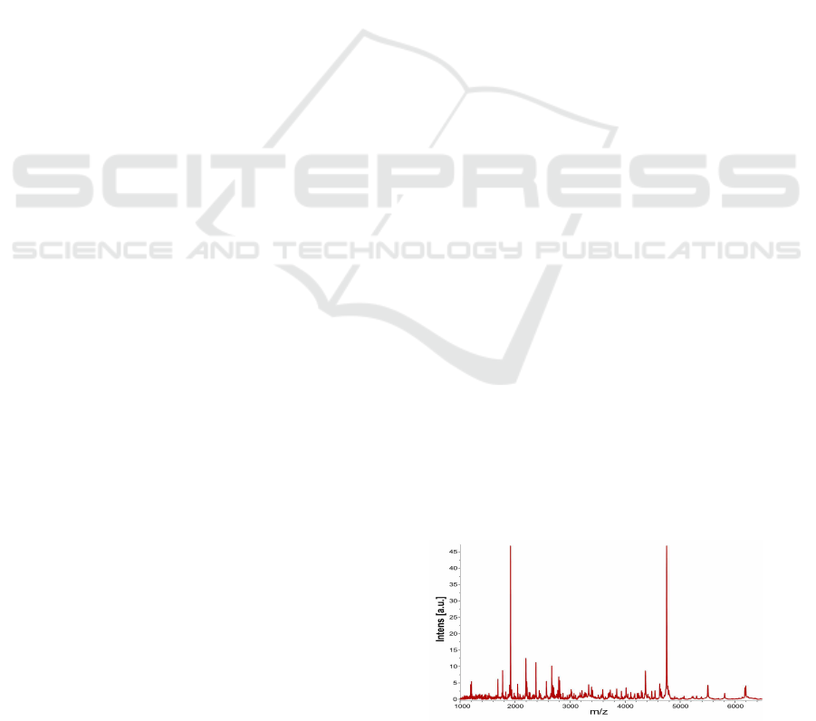
Figure 1: A typical protein/peptide proﬁle.

resulting measurements are often displayed as a graph

– a protein/peptideproﬁle (Fig. 1), in which each peak

(or signal) identiﬁes the pair of values given by the

intensity (related to the abundance) of a molecule (y–

axis) with its speciﬁc molecular mass-to-charge ra-

tio (x–axis). The ﬁnal interest in handling the huge

amount of data produced from these analyses is to pe-

251

Zoppis I., Borsani M., Gianazza E., Chinello C., Rocco F., Albo G., M. Deelder A., E. M. van der Burgt Y., Antoniotti M., Magni F. and Mauri G..

ANALYSIS OF CORRELATION STRUCTURES IN RENAL CELL CARCINOMA PATIENT DATA.

DOI: 10.5220/0003856702510256

In Proceedings of the International Conference on Bioinformatics Models, Methods and Algorithms (BIOINFORMATICS-2012), pages 251-256

ISBN: 978-989-8425-90-4

 2012 SCITEPRESS (Science and Technology Publications, Lda.)

rceive which peaks are associated with some speciﬁc

factors of interest (e.g., studying differentially ex-

pressed peaks between case and control groups) and

thus, to suggest potential biomarkers for future anal-

ysis (Latterich et al., 2008). However, to our knowl-

edge, most of these studies omit to consider the fol-

lowing key-points.

Constrained Classiﬁcation. Case / Control discrim-

ination requirements for real-world problems are

often constrained by a given true positive or false

positive rate to ensure that the classiﬁcation error

for the most important class is within a desired

limit.

Relational Information. Many domains are best de-

scribed by relational models in which instances of

multiple types are related to each other in com-

plex ways – see for example (Getoor and Taskar,

2007). In this case, some features of one entity are

often correlated with features of related entities.

It is intuitive that, just as some features are not

helpful for mining data sets, some relations might

provide informations for clustering or classiﬁca-

tion algorithms. When it comes to analyze differ-

entially expressed peaks in a case/control classi-

ﬁcation problem, comparisons are generally per-

formed between protein/peptide proﬁles of differ-

ent groups – or between statistics summarizing

the peaks’ property of a group, (Solassol et al.,

2006). Actually, different neighborhoods in the

m/z spectra can be (anti)correlated each other

and, this property, in turn, may change from group

to group. In such a situation, the incorporation

of relational information may increase the perfor-

mance of the system for “difﬁcult” data sets.

In order to manage the aboveissues, we formulate our

framework as follow.

1. The constrained classiﬁcation is met following a

standard test of hypothesis approach. This way,

one must decide between a null hypothesis and an

alternative hypothesis. A level of signiﬁcance α

(called the size of the test) is imposed on the false

alarm probability (type I error), and one seeks a

test that satisﬁes this constraint. The experimen-

tal design which derive from this formulation pro-

vide us with a tool for detecting regions of the pro-

teomic spectra characterized by properties differ-

entially expressed from group to group. Speciﬁ-

cally, in these region correlations between signals

are a “powerful” discrimination factor between

groups. This detection is our primary interest in

this paper.

2. Relational informations are introduced by giving

new graph representations for the observed sam-

ples. This way, as is used to represent relation-

ships of many interacting entities, we express cor-

relations between signals in the m/z spectra of

a patient group. Throughout, we call these rep-

resentations correlation structures (shortly, tem-

plates). Arguments of our hypotheses state con-

jectures over speciﬁc graph (i.e., template) prop-

erties. Therefore, by testing hypotheses over

properties, we can decide whether these graphs

have been changed from control to case groups

(i.e, either ccRCC or non-ccRCC groups).

Given the above concerns, this paper is laid out as

follows. In sections 2 we introduce the preliminaries

and notations. In section 3 we formulate the problem.

In section 4 we report the clinical setting and some

numerical results. Finally, in section 5 we conclude

the paper by discussing some issues of this work.

2 BASIC DEFINITIONS AND

NOTATION

Graphs are important structures to model a wide range

of natural phenomena, particularly when one has to

represent complex systems of interactions among en-

tities. Throughout this paper G = (V

∪V

,E) de-

notes a oriented bipartite graph; that is, V

and V

are two sets of vertices such that the set of all arcs

E ⊆V

×V

connect vertices in one set with vertices

in the other: i.e., E is a set of ordered pairs (v

)

with v

∈ V

and v

∈ V

constrained to not contain

any of the arcs (v

) and (v

). Given an oriented

bipartite graph G = (V

∪V

,E), the subgraph of G

given by

G = (

E), with

A ⊆ V

∪V

and

E ⊆ E is

a biclique if, for all v

∈ (

A ∩V

) and v

∈ (

A ∩V

)

then (v

) ∈

E. Biclique are, therefore, “extreme”

forms of highly inter-connected bipartite graphs and

they will of interest in deﬁning indexes for our anal-

isys. The number of vertexes N

= |V

∪V

| and the

number of arcs N

= |E| are generally called the or-

der and the size of the graph. Moreover, graphs can

be, generally, “summarized” in a compact way by var-

ious graph properties. Among all the properties in

literature (Brandes and Erlebach, 2005), here we fo-

cus on cohesion. A well known index to characterize

this notion is that of density. We treat the subject in

order to give a “local” scale of characterization for

it. While, in general, with a “global” density, we can

characterize the cohesion on the whole graph, with a

local density index as we will deﬁne below, we wish

to analyze the cohesion (i.e., by testing hypotheses),

on differently located parts of the graph. Before in-

troducing formally this notion we give the following

deﬁnition.

BIOINFORMATICS 2012 - International Conference on Bioinformatics Models, Methods and Algorithms

252

Deﬁnition 1 (Neighborhood). Let G = (V

∪V

,E)

be an oriented bipartite graph with V

two well-

ordered sets of vertexes. We call M

i, j,k

(G) = (

a (i, j,k)−neighborhood (or simply, a neighborhood

i, j,k

centered in (v

)) the subgraphs of G induced

A =

i,k

∪

j,k

where

i,k

= {v

i−k

,...,v

i+k

}

and

j,k

= {v

j−k

,...,v

j+k

}

We are now able to give the following deﬁnition.

Deﬁnition 2 (Local Density). Let G = (V

∪V

,E)

be an oriented bipartite graph and M

i, j,k

= (

E) a

neighborhood of size S centered in (v

), we deﬁne

the local density of G in M

i, j,k

den(M

i, j,k

) =

i,k

j,k

. (1)

The local density is based on the ratio of the number

of arcs among a subset of vertices to the total num-

ber of possible arcs. This way they provide a measure

of “how close” M

i, j,k

is to being an oriented biclique.

Since our primary interest is to detect which regions

of the spectra express different properties from con-

trol to case group (in our case, correlation structure

properties) we stress this point with the following def-

inition.

Deﬁnition 3 (Bipartite Graph Region). Let G = (V

∪

,E) be an oriented bipartite graph with V

two

well-ordered sets of vertexes. We say that S is a re-

gion of G if it is the subgraph S = (

∪

E) induced

through the two sequences of vertexes

and

For a formal point of view, deﬁnition 3 says nothing

more than S is a subgraph induced by a set of ver-

texes. We give this deﬁnition purely as a matter of

convenience to point out that any region of the pro-

teomic spectra (i.e., a sequence of mass-to-charge ra-

tio values) is represented here through the region of a

bipartite graph. We use widely this term in section 3

to formulate our testing procedures.

3 PROBLEM FORMULATION

In this section we formally deﬁne the problem inside

the standard test of hypotheses framework. The sub-

jects of our formulation are tests concerning graphs

properties which can be easily obtained from the fol-

lowing new samples representations. We start by

considering a population of interest divided into two

groups; respectively case and control subjects. This

population expresses the signal intensity values ob-

servable in different regions over the spectra. We

We also refer to the pair (v

) and the constant k as,

respectively, the center and the ray of the neighborhood

sample and represent each population group through

graphs which provide the observed signal correlation

structure as will be deﬁned below in section 3.1. This

way, graphs establish abstract frames of reference in

our analysis giving the opportunity to test hypothe-

ses over their properties (section 3.2). In other terms,

changes are detected by testing graph property mod-

iﬁcations from group to group. The whole procedure

provide the mass-to-charge Dalton ranges bounding

the regions where signiﬁcant changes have been de-

tected.

3.1 Correlation Structure

Representation

As is used to represent structures of many interact-

ing entities, we can express correlations inside pa-

tients’ groupsthrougha graph whose vertexesare spe-

ciﬁc mass-to-charge ratios and arcs “express” corre-

lations between signal intensities with these speciﬁc

mass-to-charge values. We call the resulting represen-

tation, the (observed) correlation structure (brieﬂy,

template). More formally, we denote the groups of

control and case subjects with I

ctrl

and I

case

respec-

tively. We assume that each group (for instance I

ctrl

)

can be expressed through a product I

ctrl

×I

ctrl

×...×

ctrl

of spaces I

ctrl

, i ∈ [n]

, given by all potential in-

tensity values whose mass-to-charge ratio is m

. We

also assume that each I

ctrl

is endowed with a distribu-

tion function f

ctrl

. More in general, let us give the fol-

lowing deﬁnition for any group of patients g on which

is deﬁned a distribution f

Deﬁnition 4 (Template). By sampling from each

pair ( f

, f

), with i ∈ [n], j ∈ [n], two sets of

i.i.d. random variables {I

i,1

i,2

,...,I

i,n

} and

j,1

j,2

,...,I

j,n

}, we call template (of g) the bi-

partite graph R

= (V

∪V

,E) with vertexes V

,...,m

} and V

= {m

′

,...,m

′

}. More-

over, (m

′

) ∈ E only if the absolute value of the

Pearson’s correlation coefﬁcient exceeds a threshold

δ. That is,

i, j

∑

k=1

i,k

−

)(I

j,k

−

)

∑

k=1

i,k

−

)

∑

k=1

j,k

−

)

≥ δ,

(2)

where

and

are the sample means.

Notice that, given the template R

= (V

,E)

and any region S of R

, we can easily provide a set of

We use the bracket notation [n] to denote the set

{1,...,n} of the ﬁrst n positive integers.

ANALYSIS OF CORRELATION STRUCTURES IN RENAL CELL CARCINOMA PATIENT DATA

253

Figure 2: The bipartite graph for RCC data (template) with

one region and two neighborhoods.

densities { d

,...,d

} by observing a set of neigh-

borhoods in S. For example, in Fig. 2 is reported

a subgraph of R

with one region and two neigh-

borhoods M

and M

Yet it is clear that, these

neighborhoods provide the set of local density val-

ues D

= {den(M

),den(M

)}. We assume that D

are observations from a distribution (of densities) re-

ferred to the region S. Throughout, we will consider

for any pair of templates R

ctrl

and R

case

the set of den-

sities D

ctrl

and D

case

as samples of observations real-

ized in a common region S to test local hypotheses

over a (density) population.

3.2 Hypothesis Testing

We recall that, statistical hypotheses (noted as H

and

) are competing statements concerning the popu-

lation parameters. The rationale for establishing our

hypotheses is deciding whether a pathology (for in-

stance, ccRCC) has modiﬁed the cohesion of a control

group’s correlation structure. Since we use density to

analyze cohesions, we should also say that for two

groups of densities, to be consistent with the above

rationale, it sufﬁces that µ

ctrl

6= µ

case

, where µ

ctrl

and

case

are the means in the control and case groups

of densities. Therefore, given (i) the (paired) sam-

ples of densities D

ctrl

= {X

,...,X

}from controls,

and D

case

= {Y

,...,Y

} from cases, (ii) their dif-

ferences D = {D

: D

= X

−Y

∈D

ctrl

∈D

case

(iii) the sample mean

D and (iv) the sample standard

deviation of difference scores S

, we can reject the

null H

: µ

ctrl

= µ

case

(no change) in favor of the alter-

native H

: µ

ctrl

6= µ

case

using

T =

√

(3)

as test statistic which, in turn, follows a Student’s t-

distribution with n−1 degree of freedom if H

is true.

For sake of clarity to specify the group g from which

the neighborhood M is drawn, we also use the notation M

Thus, we apply a classical two-sample, paired t-test,

rejecting the null when the realization t of the statistic

in expression 3 is such that |t| > t

1−α/2

(n−1), where

1−α/2

(n−1) is the quantile of Student’s t-distribution

with n −1 degrees of freedom. As argued above, the

use of local densities gives us the opportunity to ana-

lyze the cohesion in different parts of the graph. This

way, we can consider different regions over the spec-

tra – through different “local statistics”, and perform

different tests. Speciﬁcally, as noted in section 3.1,

given a common region S for both (the templates)

ctrl

and R

case

, we obtain two sets of densities D

ctrl

and D

case

. As previously stated, using these data as

observations provided by sampling both the control

and the case groups in S, we are able to apply the

test H

: µ

ctrl

= µ

case

against H

: µ

ctrl

6= µ

case

for any

region S; that is, by observing different regions, we

test the cohesion modiﬁcations from group to group

in different parts of the spectra. Given the above argu-

ments, we can deﬁne different classes of case/control

tests through the following procedures:

• Control vs. ccRCC Tests (Noted as CVR Tests).

1. We represent R

ctrl

by sampling from each

pair ( f

ctrl

, f

ctrl

) – in the control group, the

sets of i.i.d rvs {I

ctrl

,...,I

ctrl

} and

ctrl

,...,I

ctrl

2. We represent R

rcc

by sampling from each

pair ( f

rcc

, f

rcc

) – in the ccRCC group, the

sets of i.i.d rvs {I

rcc

,...,I

rcc

} and

rcc

,...,I

rcc

3. Given any region S, common both to R

ctrl

and R

rcc

, we obtain the local densities D

ctrl

{den(M

ctrl

),den(M

ctrl

),...,den(M

ctrl

)} and

rcc

= {den(M

rcc

),den(M

rcc

),...,den(M

rcc

)}.

Then for each S, we employ these sets (as ob-

servations from a density population) together

with Eq. 3 (as test statistic) in the following

tests: H

: µ

ctrl

= µ

rcc

Vs. H

: µ

ctrl

6= µ

rcc

where µ

ctrl

and µ

rcc

are, respectively, the (pop-

ulation) means of the densities in the control

and ccRCC groups.

• Control vs. Non-ccRCC Tests (CVNR Tests).

1. We represent R

ctrl

by sampling from each

pair ( f

ctrl

, f

ctrl

) – in the control group, the

sets of i.i.d rvs {I

ctrl

,...,I

ctrl

} and

ctrl

,...,I

ctrl

2. We represent R

nrc

by sampling from each

pair ( f

nrc

, f

nrc

) – in the non-ccRCC group,

the sets of i.i.d rvs {I

nrc

i,1

nrc

i,2

,...,I

nrc

i,n

} and

nrc

j,1

nrc

j,2

,...,I

nrc

j,n

BIOINFORMATICS 2012 - International Conference on Bioinformatics Models, Methods and Algorithms

254

3. Given any region S, common both to R

ctrl

and R

nrc

, we obtain the local densities D

ctrl

{den(M

ctrl

),den(M

ctrl

),...,den(M

ctrl

)} and

nrc

= {den(M

nrc

),den(M

nrc

),...,den(M

nrc

)}.

Then for each S, we employ these sets (as ob-

servations from a density population) together

with Eq. 3 (as test statistic) in the following

tests: H

: µ

ctrl

= µ

nrc

Vs. H

: µ

ctrl

6= µ

nrc

where µ

ctrl

and µ

nrc

are, respectively, the means

of the densities in the control and non-ccRCC

population groups.

• ccRCC vs. non-ccRCC Tests (RVNR Tests).

1. We represent R

rcc

by sampling from each

pair ( f

rcc

, f

rcc

) – in the ccRCC group, the

sets of i.i.d rvs {I

rcc

,...,I

rcc

} and

rcc

,...,I

rcc

2. We represent R

nrc

by sampling from each

pair ( f

nrc

, f

nrc

) – in the non-ccRCC group,

the sets of i.i.d rvs {I

nrc

i,1

nrc

i,2

,...,I

nrc

i,n

} and

nrc

j,1

nrc

j,2

,...,I

nrc

j,n

3. Given any region S, common both to R

rcc

and R

nrc

, we obtain the local densities D

rcc

{den(M

rcc

),den(M

rcc

),...,den(M

rcc

)} and

nrc

= {den(M

nrc

),den(M

nrc

),...,den(M

nrc

)}.

Then for each S, we employ these sets (as ob-

servations from a density population) together

with Eq. 3 (as test statistic) in the following

tests: H

: µ

rcc

= µ

nrc

Vs. H

: µ

rcc

6= µ

nrc

where µ

rcc

and µ

nrc

are, respectively, the means

of the densities in the ccRCC and non-ccRCC

population groups.

We point out that, each of the above class is char-

acterized to have the same alternative conjecture but

test statistics related to different parts of the graph.

We shall also say that, while evaluating higher perfor-

mance tests we may also observe in which regions of

the spectra there are the best chances of seeing dis-

criminative effects between alternatives.

4 CLINICAL SETTING AND

NUMERICAL RESULTS

The above analysis has been applied to samples col-

lected, after informed consent from all subjects par-

ticipating in the study, at the Ospedale Maggiore

Policlinico Foundation (Milano, Italy) using a stan-

dardized protocol. As a ﬁrst step the morning urine

midstream (100 mL) was collected in tubes. Af-

ter centrifugation at 3000 rpm for 10 minutes sam-

ples were divided into aliquots. For peptide and pro-

tein proﬁling the eluates from Weak Cation Exchange

magnetic beats extraction were automatically spotted

onto a Matrix–Assisted Laser Desorption Ionization

(MALDI) target plate. All samples were analyzed

using an UltraFlex II MALDI-TOF/TOF MS instru-

ment (Bruker Daltonics) and mass spectra were ac-

quired in positive linear mode in the m/z range of

1000-12000. ClinProTools 2.2 software (Bruker Dal-

tonics) was used for all MS data interpretation proce-

dures (Bosso et al., 2008).

4.1 Clinical Data

The samples cohort consists of 85 control subjects (58

men, 27 women) and 102 Renal Cell Carcinoma pa-

tients (64 men, 38 women). Mean age for controls

was 45 with a range of 30–68 years, while for pa-

tients 64 with a range of 33–88 years. It was possi-

ble to classify pathological group in patients affected

by clear cell (ccRCC) and other different histolog-

ical subtypes (respectively 79 ccRCC and 23 non-

ccRCC). ccRCC samples were classiﬁed according to

the 2002 TNM (tumor-node-metastasis) system clas-

siﬁcation.

4.2 Numerical Results

Before discussing the numerical results, it might be

useful to remember that the decisions of a statistical

test depends on a number of factors; e.g., the sam-

ple size, the test statistic, the signiﬁcance level and

the critical value. Moreover, we introduced new pa-

rameters which may inﬂuence the result as well; i.e.,

the threshold δ (employed for the template representa-

tion) and the neighborhood ray K. We also stress that,

in each class CVR, CVNR and RVNR (as deﬁned in

section 3.2), tests follow common conjectures (e.g.,

ctrl

= µ

rcc

and µ

ctrl

6= µ

rcc

) but they use statistics re-

ferred to different regions over the spectra. With the

above concerns in mind, we summarize the targets of

our experiments as follows.

1. For each class of tests, we evaluate (empirically)

which threshold δ, and ray K are employed to

detect the lowest number of correlation structure

changes from control to case groups. In other

terms, for different pairs of δ and K we count the

number of signiﬁcant tests rejecting the null hy-

pothesis. For this, we constrain δ to range within

a set of higher Pearson’s correlation coefﬁcients.

2. By using the values of δ and K obtained above,

we detect the mass-to-charge ratio bounds which

identify modiﬁed regions over the spectra. That

is, regions where we have detected a correlation

ANALYSIS OF CORRELATION STRUCTURES IN RENAL CELL CARCINOMA PATIENT DATA

255

structure modiﬁcation at a speciﬁc level of signif-

icance.

Indeed, we ﬁrst established a ﬁxed number of re-

gions (i.e., 7), a set of arbitrary thresholds T =

{0.75, 0.76,0.77,0.78, 0.79,0.80} and a set of arbi-

trary rays R = [6]. Then, for each combination of

δ ∈T and K ∈R, we evaluated (for each class of tests)

the number of signiﬁcant tests rejecting the null hy-

pothesis over the spectra. In tab. 1, we report, for

each class, both the pair (δ,K) employed to detect the

lowest number (i.e., n = 1) of tests rejecting the null,

and the mass-to-charge ranges which identify the re-

jection regions at a 5% signiﬁcance level.

5 CONCLUSIONS

This study showed the possibility to use the extracted

peptides to separate healthy subjects from tumor pa-

tients and mostly to distinguish non-ccRCC from

RCC. By testing hypotheses on a speciﬁc graph prop-

erty (i.e., density), we derived decision procedures

able to provide the clinical modeler with lists of Dal-

ton ranges where it has been detected distinguishing

regions. We point out that, from a clinical perspec-

tive, in order to apply this approach (for example, to

decide the membership group of new subjects), it will

be necessary to compute a correlation matrix (whose

components are given by Eq. 2) over a set of techni-

cal replicates. This will be the most obvious extension

for our next work when new (biological and technical)

samples will be available. Moreover, we can sum-

marize, as follow, some further extensions which we

are immediately interested to: (I) We need to deter-

mine conclusively the identity of the lists of signals

in any differentially expressed region. The theoret-

ical framework of section 3 was employed to detect

spectral signals for their biological importance (for

instance, to suggest potential biomarkers for future

analyses) even their identity is not yet ensured. Identi-

ﬁcation of the peptides/proteins, generating these sig-

nals, is a very laborious process implying the analy-

sis of the urine extract with different MS approaches.

Therefore, in order to recognize candidate multiple

biomarkers, for a speciﬁc disease, it’s important ﬁrst

to determine their diagnostic “power” and then to in-

vestigate better their biological role in the disease

Table 1: Mass-to-Charge regions for Control vs. Case.

CVR CVNR RVNR

δ = 0.75, K = 2 δ = 0.75,K = 2 δ = 0.75,K = 2

From To From To From To

1719 2084 1719 2084 4625 5374

mechanisms. (II) The dominant approach to classi-

ﬁer design in clinical studies has been to minimize the

probability of error – see for example, (Dudoit et al.,

2002). Yet it is clear that failing to detect a malignant

tumor has drastically different consequences than er-

roneously ﬂagging a benign tumor. In other words,

classiﬁcation requirements are often constrained by a

given true positive (type I error) and false positive rate

(type II error) to ensure that the classiﬁcation error

for the most important class is within a desired limit.

In order, for our procedures to take into account all of

these two requirements, it is necessary to constrain the

type II error. We point out that, here by constraining

only the type I error, we applied a methodology ap-

proach mainly to provide the list of modiﬁed regions.

ACKNOWLEDGEMENTS

This work was supported by grants of the Ital-

ian Ministry of Research: PRIN 2006, FIRB 2007

(RBRN07BMCT

11), FAR 2006–2011, and in part

by both the EuroKUP COST Action (BM0702) and

the NEDD project of the “Regione Lombardia”.

REFERENCES

Bosso, N., Chinello, C., Picozzi, S., Gianazza, E., Mainini,

V., Galbusera, C., Raimondo, F., Perego, R., Casel-

lato, S., Rocco, F., Ferrero, S., Bosari, S., Mocarelli,

P., Kienle, M. G., and Magni, F. (2008). Human urine

biomarkers of renal cell carcinoma evaluated by clin-

prot. Proteomics - Clin. App., 2:1036–1046.

Brandes, U. and Erlebach, T., editors (2005). Network Anal-

ysis: Methodological Foundations, volume 3418 of

Lect. Notes in Computer Science. Springer.

Brannon, A. and Rathmell, W. (2010). Renal cell carci-

noma: where will the state-of-the-art lead us? Curr.

Oncol. Rep., 12:193–201.

Drucker, B. (2005). Renal cell carcinoma: current status

and future prospects. Cancer Treat. Rev., 31:536–545.

Dudoit, S., Fridlyand, J., and Speed, T. (2002). Compari-

son of discrimination methods for the classiﬁcation of

tumors using gene expression data. J. of the American

Stat. Assoc., 97(457):77–87.

Getoor, L. and Taskar, B. (2007). Introduction to Statistical

Relational Learning. The MIT Press.

Latterich, M., Abramovitz, M., and Leyland-Jones, B.

(2008). Proteomics: New technologies and clinical

applications. Eur. Jour. Cancer., 44:2737–2741.

Solassol, J., Jacot, W., Lhermitte, L., Boulle, N., Maude-

londe, T., and Mang, A. (2006). Clinical proteomics

and mass spectrometry proﬁling for cancer detection.

Expert Rev. Proteomics, 3(3):311–320.

BIOINFORMATICS 2012 - International Conference on Bioinformatics Models, Methods and Algorithms

256