REAL TIME OBJECT TRACKING ON GPGPU

∗

Maciej Chociej and Adam Polak

Theoretical Computer Science Department, Faculty of Mathematics and Computer Science, Jagiellonian University,

Krak

ow, Poland

Keywords:

Motion Tracking, GPGPU, Optical Flow, Foreground Separation.

Abstract:

We propose a system for tracking objects in a video stream from a stationary camera. Our method, as of-

ten used, involves foreground-background separation and optical ﬂow calculation. The major ﬁnding is fast

feedback process that leads to an accurate detection of background-object and object-object boundaries and

maintaining them during object occlusions. The contribution of this paper also includes improvements to com-

puting dense optical ﬂow and foreground separation. The methods described were implemented on a GPGPU

and yield performance results sufﬁcient for real time processing. Additionally, our approach makes no a priori

assumptions on the characteristics of tracked objects and can be utilized to track both rigid and deformable

objects of various shapes and sizes.

1 INTRODUCTION

Object tracking is one of central problems in com-

puter vision. Robust tracking algorithms need to com-

bine techniques from many areas of the ﬁeld. Ques-

tions that need to be answered are:

• what are the objects we want to track;

• what are the cues that allow us to separate an ob-

ject of our interest from its surroundings;

• what abstractions to model an object with and how

to maintain their correspondence in time.

Even more questions arise when motion is taken into

account:

• how to detect movement accurately and fast in

terms of computation time;

• how should detection of movement inﬂuence the

way we partition objects in the image space;

• can we through motion analysis distinguish be-

tween objects that are involved in complicated,

dynamic interactions.

The literature on the subject is vast and presents many

methods that respond to most of these questions. In

a recent survey (Yilmazr et al., 2006) tracking algo-

rithms are divided based on the representation of the

∗

This paper is based on work funded by Polish Ministry

of Science and Higher Education (grant R00 0081 11) in

cooperation with AutoID Polska S.A.

objects as: a single point or points, simpliﬁed geo-

metric shapes, object contours and silhouettes and ar-

ticulated shape models constructed from the former

types. In (Bugeaue and P

erezz, 2008) the authors

reassign those algorithms to three distinct groups:

detect-before-track, track and combine partitions and

the third group: track distinct features or feature dis-

tributions. The ﬁrst type of algorithms relies on ex-

ternal schemes that detect classes of well known ob-

jects (license plates (Donoser et al., 2007)(Zweng

and Kampel, 2009), vehicles (Feris et al., 2011), hu-

mans and human faces (Karlsson et al., 2008)(Wu and

Nevatia, 2007) and describe them in terms of simple

structures like points or bounding boxes, which then

can be tracked over time. The second type is based

on a primary detection of objects, possibly by exter-

nal means. Such objects silhouettes, usually repre-

sented by the contour or an energy function in the im-

age space, are then evolved to meet speciﬁc energy

preservation criteria. The last group consists of al-

gorithms focusing on the detection and tracking of

unique features in the appearance of the objects and

by their movement predicting and extrapolating the

movement of an object as a whole.

The paper (Bugeaue and P

erezz, 2008) contains

an interesting review of those three types of algo-

rithms, their strengths and drawbacks and proposes

a hybrid method combining those approaches. Our

method is based on similar premises, but varies sig-

niﬁcantly in details. By exploiting the power of GPG-

303

Chociej M. and Polak A..

REAL TIME OBJECT TRACKING ON GPGPU.

DOI: 10.5220/0003862303030310

In Proceedings of the International Conference on Computer Vision Theory and Applications (VISAPP-2012), pages 303-310

ISBN: 978-989-8565-04-4

 2012 SCITEPRESS (Science and Technology Publications, Lda.)

PUs we compute dense optical ﬂow that allows us

to predict object deformations with higher precision.

The quality of our optical ﬂow also makes us less de-

pendent on detecting ’observations’ (in the sense of

(Bugeaue and P

erezz, 2008)), as object identiﬁcation

can be propagated for much longer time. Finally in

(Bugeaue and P

erezz, 2008) object distinction is per-

formed via multiple graph-cuts, whereas we employ

a delayed voting scheme. In the scenario with a sta-

tionary camera this allows us to process high resolu-

tion inputs with real-time performance and compara-

ble accuracy.

It is worth to mention that there exist another ap-

proach to combine the three mentioned types of algo-

rithms, i.e. data fusion (Makris et al., 2011).

2 THE PROBLEM

In this paper we propose a method that can be used

to solve the following basic problem: In each frame

of a given video stream we want to separate moving

objects and assign to them unique identiﬁers. These

identiﬁers should be discovered as soon as the object

appears in the view and should be held as long as the

object is visible.

An additional goal is to strike a proper balance be-

tween the precision and the computational cost. We

strove for real-time performance and thus decided to

focus on algorithms where natural data parallelism in

the image space could be exploited.

Our method is intended to work at the lowest level

of a more complex tracking system. It is designed to

be easily integrated with higher level logic capable of

handling more difﬁcult object-object interactions.

We deﬁne an object as a group of pixels forming

a connected component of the input image and mov-

ing in a coherent way. We do not make any other

assumptions about tracked objects. This makes our

method general and versatile, capable of tracking hu-

mans in motion, vehicles, as well as other moving ob-

jects, both rigid and deformable. However, we require

that the camera is stationary and that it is, without los-

ing generality, in an upright orientation.

When tracking the objects we face the following

major problems which need to be solved:

• detecting new objects, and separating them from

the background;

• resolving object occlusion;

• separating objects which move together in close

proximity in the same direction;

• splitting objects which we incorrectly tracked as a

single one;

• joining objects which we detected separately but

seem to be parts of one physical entity.

We have implemented our method on multicore CPUs

and CUDA based GPGPUs and performed extensive

tests that included footage from various indoor and

outdoor scenarios. These tests had shown that our

approach handles with reasonable accuracy all these

cases, apart from the last one – joining object parts.

We leave this to be solved with higher level logic,

which is the goal of our future work.

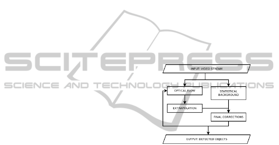
3 METHOD OVERVIEW

The main modules our method consists of are pre-

sented in the ﬁgure below. It is followed by the gen-

eral description of these modules.

Figure 1: Block diagram of our method.

Our procedure processes consecutive frames ap-

pearing in the video stream. After the frame is pro-

cessed we return its partition into a number of tracked

objects and the background.

When the new frame appears in the video stream,

we process it as follows:

1. Optical Flow. We compute the optical ﬂow be-

tween the previous and the current frame. The

method we use exploits the object partition com-

puted for the previous frame.

2. Extrapolation. We predict the location of tracked

objects in the current frame using the computed

optical ﬂow and the previous frame.

3. Statistical Background. We compute the

foreground-background separation in the current

frame based on statistical model of the back-

ground.

4. Final Corrections. We apply small corrections

to the extrapolated partition from the second step.

These include:

VISAPP 2012 - International Conference on Computer Vision Theory and Applications

304

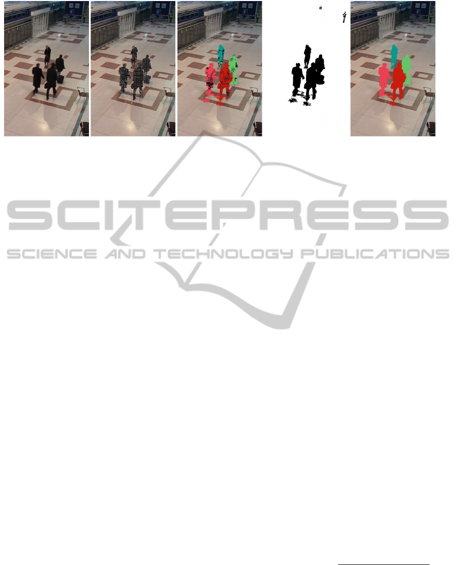
Figure 2: An example frame from the PETS 2006 dataset, left to right: the original frame, the optical ﬂow, the extrapolation,

the foreground, the ﬁnal object partition.

• splitting objects that are not coherent anymore;

• detecting new object that appeared for the ﬁrst

time in the current frame;

• assigning IDs to pixels which are in the

foreground according to the foreground-

background separation but have no IDs

reasoned from the extrapolation phase.

The algorithms we devise to complete these steps are

described in details in the next section.

4 ALGORITHMS

4.1 Optical Flow

The optical ﬂow pass we use is a block matching al-

gorithm organized in a coarse-to-ﬁne way similar to

the well known Bouguet’s (Bouguet, 2000) imple-

mentation of the Lucas–Kanade window registration

scheme (Lucas and Kanade, 1981). This method had

been often discarded in application to dense optical

ﬂow due to complications that arise when tracking ob-

jects with low texture or frequent occlusions. By care-

fully choosing appropriate features to track one can

limit the negative inﬂuence of the aperture problem,

but this in general results in sparse optical ﬂow esti-

mation (Tomasi and Kanade, 1991)(Shi and Tomasi,

1993). Other methods incorporate many ways to in-

troduce a global constraint of smoothness (Horn and

Schunck, 1981). This solves the aperture problem but

on the other hand tends to distort information where

ﬂow discontinuities appear. It is also computation-

ally more expensive as global constraints arise and

the solution cannot be tackled locally. State of the

art optical ﬂow algorithms (Bruhn et al., 2005)(Xu

et al., 2010) exploit both these ideas with great ac-

curacy, but are prohibitively slow and do note seem

to ﬁt for GPGPU architectures. In order to compute

dense optical ﬂow with attention to ﬁne object silhou-

ette tracking we introduced improvements to the pyra-

midal scheme of (Bouguet, 2000).

4.1.1 Basic Deﬁnitions

The optical ﬂow algorithm processes the two consec-

utive images from the video stream L, C and an iden-

tiﬁer map ID that contains the object partition of L.

The output consists of a matrix of size width × height

containing pairs: (u, v) ∈ Z

of displacements com-

puted for each pixel that belongs to an object.

In the ﬁrst step two pyramids of image miniatures are

created for L and C. Let us denote these image minia-

tures by L

and C

(0 ≤ i ≤ l). Each of the l + 1 lev-

els is a matrix containing extended pixel touples, each

level half the width and half the height of the previ-

ous. We will refer to the level 0 as the top and to the

level l as the bottom. The extended pixel touples con-

tain three values representing the color components r,

g, b and two additional values h and v for the horizon-

tal and vertical gradient values. In order to downsize

the images we use a small Gaussian kernel. An aux-

iliary pyramid of identiﬁers, denoted ID

, is created

from the ID map. The selection of the pixel’s identi-

ﬁer is performed by choosing the most frequent iden-

tiﬁer from the four pixels directly above in the higher

pyramid level.

For the window registration algorithms we will use

a normalized dissimilarity measure, based on a

componentwise L

norm, that compares pixels’ r-

neighborhoods (for a given radius r).

, p

) =

∑

v∈{−r,...,r}

kI[p

+ v] − J[p

+ v]k

(2r + 1)

(1)

4.1.2 Self-dissimilarity

The aperture problem arises most commonly from the

appearance of two types of regions in the analyzed

REAL TIME OBJECT TRACKING ON GPGPU

305

images: large spots with low or none texture (e.g.

solid blocks of one color) and regions with repeat-

ing self-similar patterns (e.g. a checkered fabric of

ones clothing). The dissimilarity between windows

on consecutive frames is low and near constant in the

local neighborhood or has multiple regular minimums

in those parts of the image. This leads to random op-

tical ﬂow estimation when we minimize the dissimi-

larity in order to ﬁnd the proper window registration.

To prevent such behavior we must ﬁrst detect which

regions hold those unwanted properties. For a given

radius r we deﬁne a pixel’s self-dissimilarity as:

(p) =

∑

v∈{−r,...,r}

(p, p + v) (2)

This quantity tells us weather a pixel’s local neighbor-

hood is similar to many such neighborhoods in near

proximity. High self-dissimilarity implies the pix-

els neighborhood is unique, low self-similarity hints

us that the pixels neighborhood might be mistaken

by a similar neighborhood nearby. Our experiments

have shown that in the areas of low self-dissimilarity

the standard unmodiﬁed optical ﬂow algorithm often

ﬁnds illusionary movement where none has actually

happened, or detects no movement where there has

been some. The choice of using average dissimilarity

rather than minimum was based on experiments con-

ducted. The minimum of dissimilarities was much

more inﬂuenced by image noise and resulted in less

informative level sets.

For a given limit of dissimilarity lim we compute a

pyramid of matrices SD

matching the sizes of the im-

age and ID pyramids, that contains self-dissimilarity

information from the pyramid L

. We start at the bot-

tom and proceed to the top. The resulting level-0

self-dissimilarity map SD

describes the regions of

the image in terms of susceptibility to the aperture

problem. A level-0 pixel (i.e. SD

[x, y] = 0) has local

neighborhoods in every image in the image pyramid

at least lim dissimilar. Similarly: a level k pixel (i.e.

[x, y] = k) has dissimilarity at least lim in the pyra-

mid levels l up to k.

4.1.3 Window Scaling and Object Masking

Our algorithm will utilize a registration windows of

different sizes. We incorporate the scaling factor c

into the dissimilarity measure d

(c, p

, p

) =

∑

v∈{−r,...,r}

kI[p

+ cv] − J[p

+ cv]k

(3)

Moreover, in order to improve the accuracy of the

window registration in regions with motion occlusion

we decided to incorporate an additional constraint to

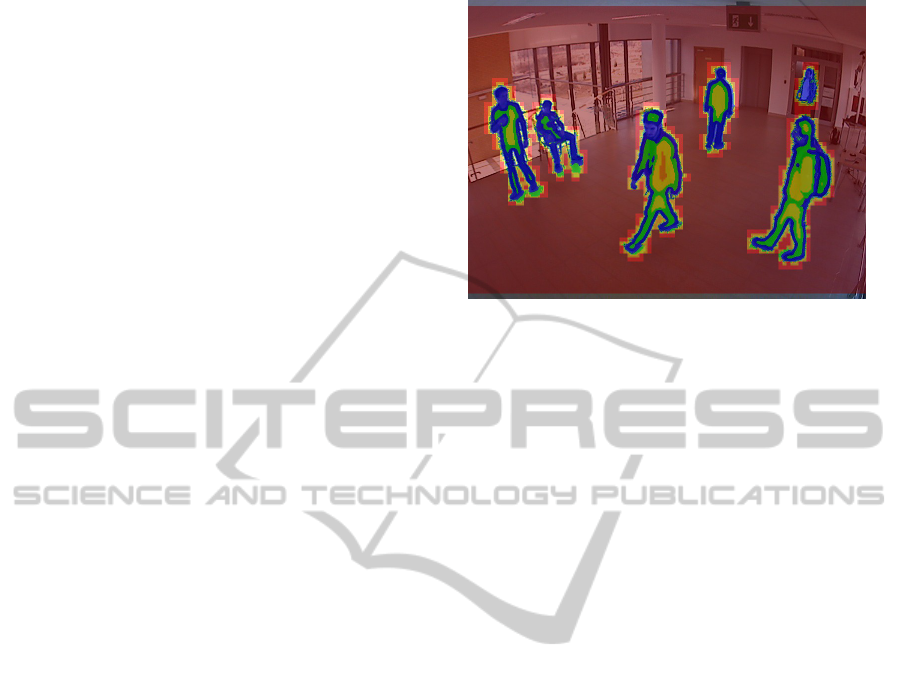
Figure 3: The self-dissimilarity map: pixel values ranging

from 0 (blue) to 5 (red).

the dissimilarity measuring function. Optical ﬂow

methods like (Sun et al., 2010) try to segment the im-

age based on coherency of optical ﬂow, we use the ob-

ject assignment in a similar manner. For a given pixel,

we take into account only those pixels from it’s neigh-

borhood that belong to the same object. If a pixel has

an ID set (and only those are processed when com-

puting the optical ﬂow) we consider only those pixels

from the r-neighborhood that share the same ID.

4.1.4 Coarse to Fine Window Registration

In the main part of our optical ﬂow algorithm we

ﬁnd the displacements with a dynamic window reg-

istration approach. Similar concept of adaptive win-

dow sizes and shapes has been mentioned in (Kanade

and Okutomi, 1994)(Yang et al., 2004). In the fol-

lowing we will use a new variable s which is to be

ﬁxed afterwards due to some experiments. At each

level we limit ourselves to integer displacements can-

didates v ∈ {−1, 0, 1}

. With l + 1 pyramid levels this

results in maximal displacements of 2

in total. At

the bottom, for every pixel we choose s best displace-

ments that minimize the dissimilarity between the lo-

cal neighborhoods in the consecutive frames. At lev-

els l − 1 through 0 we utilize the s best candidates

from the level directly below as starting offsets for the

displacement vectors. We use the self-dissimilarity

map to scale the window when required. If process-

ing a pixel that has the self-dissimilarity level higher

than the currently processed pyramid level we need to

make the window larger.

For performance reasons we calculate the optical

ﬂow only for the pixels where an object has been dis-

covered. Our experiments show that for the sake of

accuracy it is useful to rise the number of samples

that are compared when computing dissimilarity with

a bigger window. In most of our tests 6 levels of the

VISAPP 2012 - International Conference on Computer Vision Theory and Applications

306

image pyramid were sufﬁcient to detect the largest

displacements. Considering that a pixel at the bottom

level would represent a 32 × 32 pixel square at the

highest resolution, we increase the number of sam-

ples in the d

dissimilarity measure by a factor of 4

up to 16.

The nature of the other components in the tracker

allows us to limit the search to integer displacements.

Most differential optical ﬂow algorithms ﬁnd dis-

placements with sub-pixel precision. This often re-

quires bilinear interpolation as pixel values need to be

resolved at real coordinates. Our experiments have

shown that s = 3 not only compensates this lack of

precision in the lower levels, but in fact often gives

better results.

Figure 4: Behavior of optical ﬂow algorithms on regions

with low texture: left – pyramidal LK, right – our method.

4.2 Extrapolation

The main task of this algorithm is to predict where

objects detected in the previous frame are going to ap-

pear in the current one. We do this in a rather straight-

forward manner. To extrapolate a location of an ob-

ject we process all pixels belonging to it and trans-

late them by vectors computed during the optical ﬂow

phase. Apart from the object partition, from the pre-

vious frame we get the conﬁdence value in each pixel.

During the extrapolation phase we will extrapolate

them as well, while the section 4.4 will elaborate in

detail on how these conﬁdence values are initiated in

the ﬁrst place. After some experiments we have de-

veloped two heuristics which improve the quality of

the extrapolation.

The optical ﬂow computed using our method falls

victim to some irregularities and in each frame a frac-

tion of pixels is extrapolated in the wrong direction.

To prevent this, we check for each pixel whether it’s

optical ﬂow vector is close enough to the average opti-

cal ﬂow calculated in the pixel’s neighborhood. If this

condition fails we do not extrapolate the given pixel

at all.

Two pixels from the previous frame (possibly be-

longing to two different objects) can be extrapolated

to the same pixel in the current frame. It means that

one object occludes another and we need to decide

which of them is closer to the camera. In order to

resolve this we assume, without losing of generality,

that the camera is in an upright orientation. Thus we

assume that an object located lower in the image is

also closer. This method performs ﬁne when object

movement is limited to a plane, or close to a plane.

Many surveillance scenarios allow such an assump-

tion. More complicated tracking cases, where the ob-

jects can move freely in all three dimensions, would

require a different method.

4.3 Statistical Background/Foreground

Detection

In order to reinforce the information coming from the

extrapolation phase we detect foreground objects by

analyzing statistical properties of the video stream.

The foreground detection module maintains a long

term model of the background that contains the color

value mean and standard deviation for each pixel.

Apart from the long term model we keep two short

term statistics (mean and standard deviation) that are

gathered over the span of a limited number of frames

(say, by 0.5 sec). The long term color statistics are

used to decide weather a pixel from a new frame

belongs to the foreground. The short term parame-

ters inform us about the volatility of the pixel, which

is used to determine the background learning speed.

Additionally, we forbid changes to the background

model in the regions where the extrapolation phase

has already predicted an object.

The short term parameters are updated componen-

twise, by means of a moving average, with a constant

rate every time a new frame appears. The rate is high

(i.e. 0.1) in order to accumulate information over a

short period. The long term parameters are updated

componentwise with a much lower learning rate (i.e.

0.01) that also depends on the volatility of the pixel

and the contents of ID

. If volatility is high or we see

that the region belongs to an object, the learning rate

drops signiﬁcantly. If the short term parameters are

stable, we increase the long term learning rate.

In order to detect regions belonging to the fore-

ground the difference between the color values in the

frame and the background model is measured and

thresholded. The long term deviation is used to de-

termine the threshold levels. We also introduce a

constant additive and a constant multiplicative factors

that can be used to scale the deviation, and control the

background-foreground separation sensitivity.

4.4 Final Corrections

The purpose of this phase is to combine data we acq-

REAL TIME OBJECT TRACKING ON GPGPU

307

uired from the extrapolation phase and the

background-foreground separation and then uti-

lize it to introduce corrections in the predicted ID

map of the current frame.

The algorithm consists of three steps, which are

preceded by computing new foreground map. A pixel

is said to be in the foreground if it belongs to any ex-

trapolated object or the statistical foreground.

4.4.1 Splitting Objects

This step is performed to assure that every extrapo-

lated object is coherent.

First, we ﬁnd the connected components of the

foreground map. Each foreground pixel is connected

to its four neighbors and the resulting graph is a sub-

graph of a 2D-grid.

Then, for each extrapolated object we decide

which component it belongs to and remove parts of

this object from the remaining. We rank candidate

components summing conﬁdence values of pixels be-

longing to the intersection of this component and a

given object.

The parts of the object that lie outside of the high-

est ranked connected component are subtracted from

the object.

4.4.2 Detecting New Objects

In this step we detect objects that were not present on

the previous frame. These are objects that appeared in

the view at this moment or were tracked as a part of

another object and were detached from it in the previ-

ous step. If there exists a connected component that

has an empty intersection with all the extrapolated ob-

jects we assign a new unique identiﬁer to all the pixels

inside and set their conﬁdence value to 1.

4.4.3 Filling Gaps

We deﬁne a gap as a pixel which is believed to belong

to the foreground but has no identiﬁer assigned. Usu-

ally, at this stage of processing there are still such pix-

els left. We assign them to an object with a procedure

that searches the ID

map in a breadth-ﬁrst manner.

For every gap pixel (x, y) we check its eight neigh-

bors and ﬁnd the most frequent ID among them. If

this ID appears at least three times, we assign it to

this gap pixel. Pixel’s new conﬁdence is set to the dif-

ference between the average conﬁdence of neighbors

with the chosen ID and the second best. If such differ-

ence turns out to be negative, we leave the gap pixel

unchanged.

This procedure is iterated until no gap pixel

changes its identiﬁcation.

5 IMPLEMENTATION DETAILS

The methods described have been prototyped in C++

and tested on x86 CPUs. The algorithms have been

then ported to NVIDIA CUDA environment. We have

implemented the foreground separation, the optical

ﬂow, extrapolation and code related to processing the

foreground connected components on the GPU. The

only part that relies on CPU computation is the gap

ﬁxing phase that requires a breadth-ﬁrst approach.

Although there are BFS algorithms on GPGPUs we

have not decided to implement them for simplicity

reasons. The overhead related to synchronizing GPU

and CPU execution, transferring partial data and run-

ning BFS on the CPU has no major inﬂuence on over-

all performance.

The foreground separation proved to be easily par-

allelized, as pixels could be processed independently.

The optical ﬂow phase is the most time consuming

part of the algorithm, thus its efﬁcient implementa-

tion was the biggest challenge. The problem was

memory bandwidth constrained and required careful

attention when reading and writing data. A number of

approaches has been developed in order to make co-

alesced memory accesses possible. The optical ﬂow

code had a deeply nested structure that had to be prop-

erly unrolled for performance reasons. The perfor-

mance tuning of the optical ﬂow required a good bal-

ance between the shared memory usage and the num-

ber of simultaneously working blocks.

6 RESULTS

The ﬁgures at the end present the object segmentation

produced from various test scenarios. The scenario

depicted in the ﬁrst ﬁgure shows a group of 6 persons

involved in complicated occlusions. The dimensions

of the image are 800 × 600 running at 15 frames per

second. The scenarios from the two middle ﬁgures are

taken from the PETS 2006 workshop datasets. These

streams have PAL resolution (i.e. 720 × 576) and are

recorded at 25 frames per second. The last scenario

was recorded with a 960 × 640 frame size at 12.5

frames per second.

Our software run on a Tesla C2050 GPU reaches

sustained real-time performance in these scenarios.

The average frame processing time varies from 15 to

25 milliseconds. The performance is greatly depen-

dent on the optical ﬂow phase and thus on the total

area of tracked objects.

We have also tested the optical ﬂow alone on

frames in PAL resolution counting displacement vec-

tors in every pixel. The processing time of 200 mil-

VISAPP 2012 - International Conference on Computer Vision Theory and Applications

308

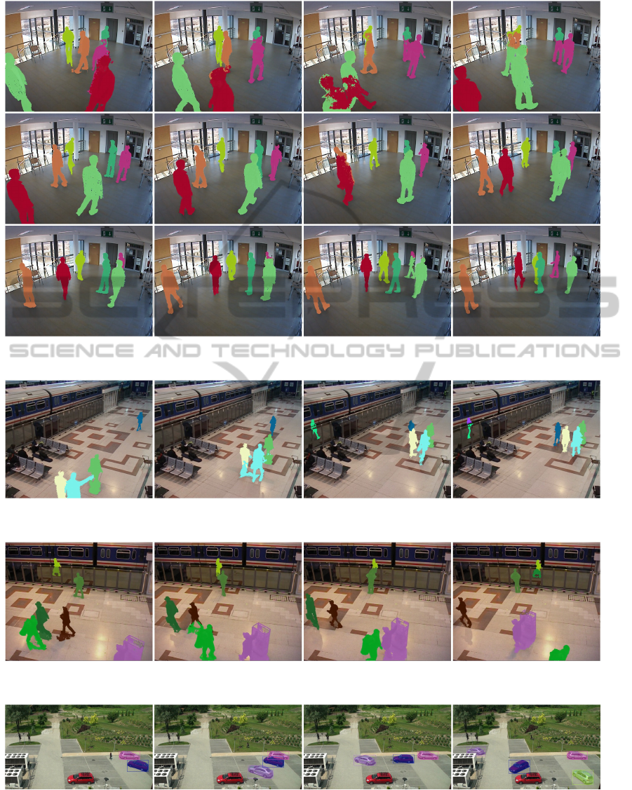
Figure 5: 6-person occlusions.

Figure 6: PETS 2006 dataset S1, camera 3.

Figure 7: PETS 2006 dataset S1, camera 4.

Figure 8: Parking lot.

liseconds is the pessimistic case we might be facing.

The prototype of our algorithms has been imple-

mented as a pure CPU solution. In simpler scenarios

(i.e. the parking lot) it reached near real-time per-

formance when run on a multicore Intel Xeon X5650

processor.

REAL TIME OBJECT TRACKING ON GPGPU

309

7 FURTHER WORK

Our tracker is a low-level solution and in order to im-

prove the detection and tracking quality higher level

logic might be implemented. In particular such logic

could observe the objects in the context of a longer

period of time, maintaining its history.

Our future work will focus on following issues:

• When a tracked person hides behind an obstacle

and then reappears it is detected as a completely

new object.

• Large number of objects appearing simultane-

ously in the stream results in lower tracking qual-

ity and performance, especially in cases with

complicated occlusions. There is need for an al-

gorithm for deciding which of the tracked objects

can be ignored (e.g. tracking only humans or ve-

hicles).

• Some surveillance scenarios include monitored

zones covered by more than one camera. Combin-

ing data from multiple trackers can lead to better

results.

With the above issues resolved our tracker to-

gether with those high level components might be

considered as an important part of a robust surveil-

lance system.

ACKNOWLEDGEMENTS

The authors would like to thank the PETS workshops

organizers for publishing the datasets we extensively

used in our tests.

REFERENCES

Bouguet, J.-Y. (2000). Pyramidal implementation of the

lucas kanade feature tracker description of the algo-

rithm.

Bruhn, A., Weickert, J., and Schn

orr, C. (2005). Lucas

kanade meets horn schunck: Combining local and

global optic ﬂow methods. International Journal of

Computer Vision.

Bugeaue, A. and P

erezz, P. (2008). Track and cut: Simul-

taneous tracking and segmentation of multiple objects

with graph cuts. Journal on Image and Video Process-

ing.

Donoser, M., Arth, C., and Bischof, H. (2007). Detecting,

tracking and recognizing license plates. In Proceed-

ings of the 8th Asian conference on Computer vision -

Volume Part II, Berlin, Heidelberg. Springer-Verlag.

Feris, R., Siddiquie, B., Zhai, Y., Petterson, J., Brown,

L., and Pankanti, S. (2011). Attribute-based vehicle

search in crowded surveillance videos. In Proceedings

of the 1st ACM International Conference on Multime-

dia Retrieval, New York, NY, USA. ACM.

Horn, B. and Schunck, B. (1981). Determining optical ﬂow.

Artiﬁcal Intelligence.

Kanade, T. and Okutomi, M. (1994). A stereo matching

algorithm with an adaptive window: Theory and ex-

periment. IEEE Trans. Pattern Anal. Mach. Intell.

Karlsson, S., Taj, M., and Cavallaro, A. (2008). Detection

and tracking of humans and faces. Journal on Image

and Video Processing.

Lucas, B. and Kanade, T. (1981). An iterative image regis-

tration technique with an application to stereo vision.

In Proceedings of the 7th International Joint Confer-

ence on Artiﬁcial Intelligence - Volume 2, San Fran-

cisco, CA, USA. Morgan Kaufmann Publishers Inc.

Makris, A., Kosmopoulos, D., Perantonis, S., and Theodor-

idis, S. (2011). A hierarchical feature fusion frame-

work for adaptive visual tracking. Image Vision Com-

put.

Shi, J. and Tomasi, C. (1993). Good features to track. Tech-

nical report, Cornell University, Ithaca, NY, USA.

Sun, D., Sudderth, E., and Black, M. J. (2010). Layered

image motion with explicit occlusions, temporal con-

sistency, and depth ordering.

Tomasi, C. and Kanade, T. (1991). Shape and motion from

image streams: a factorization method - part 3 detec-

tion and tracking of point features. Technical report,

Pittsburgh, PA, USA.

Wu, B. and Nevatia, R. (2007). Detection and tracking of

multiple, partially occluded humans by bayesian com-

bination of edgelet based part detectors. International

Journal of Computer Vision.

Xu, L., Jia, J., and Matsushita, Y. (2010). Motion detail pre-

serving optical ﬂow estimation. In Computer Vision

and Pattern Recognition. IEEE Computer Society.

Yang, R., Pollefeys, M., and Li, S. (2004). Improved real-

time stereo on commodity graphics hardware. In Pro-

ceedings of the 2004 Conference on Computer Vision

and Pattern Recognition Workshop (CVPRW’04) Vol-

ume 3 - Volume 03, Washington, DC, USA. IEEE

Computer Society.

Yilmazr, A., Javed, O., and Shah, M. (2006). Object track-

ing: A survey. ACM Computing Survey, 38.

Zweng, A. and Kampel, M. (2009). High performance im-

plementation of license plate recognition in image se-

quences. In Proceedings of the 5th International Sym-

posium on Advances in Visual Computing: Part II,

Berlin, Heidelberg. Springer-Verlag.

VISAPP 2012 - International Conference on Computer Vision Theory and Applications

310