
REGION GROWING: ADOLESCENCE AND ADULTHOOD
Two Visions of Region Growing: in Feature Space and Variational Framework
C. Revol-Muller
1
, T. Grenier
1
, J. L. Rose
1
, A. Pacureanu
1
, F. Peyrin
2
and C. Odet
1
1
CREATIS, CNRS UMR 5220, Inserm U1044, Univ. de Lyon 1, INSA-Lyon, 7 Av. Jean Capelle 69621, Lyon, France
2
ESRF, BP 220, 38043 Grenoble Cedex, France
Keywords: Region Growing, Feature Space, Scale Parameters, Variational Approach, Shape Prior Energy, Vesselness.
Abstract: Region growing is one of the most intuitive techniques for image segmentation. Starting from one or more
seeds, it seeks to extract a meaningful object by iteratively aggregating surrounding pixels. Starting from
this simple description, we propose to show how region growing technique can be elevated to the same rank
as more recent and sophisticated methods. Two formalisms are presented to describe the process. The first
one derived from non-parametric estimation relies upon feature space and kernel functions. The second one
is issued from variational framework. Describing the region evolution as a process, which minimizes an
energy functional, it thus proves the convergence of the process and takes advantage of the huge amount of
work already done on energy functional. In the last part, we illustrate the interest of both formalisms in the
context of life imaging. Three segmentation applications are considered using various modalities such as
whole body PET imaging, small animal µCT imaging and experimental Synchrotron Radiation µCT
imaging. We will thus demonstrate that region growing has reached this last decade a maturation that offers
many perspectives of applications to the method.
1 INTRODUCTION
Life imaging by means of many modalities (X-ray
Computed Tomography, Magnetic Resonance
Imaging (MRI), Ultrasounds, Positron Emission
Tomography (PET), etc.) allows a three-dimensional
exploration of the anatomical structures with an
increasingly precision and provides to the doctors or
biologists a huge amount of data to analyse. In order
to leverage these high-tech imaging systems, it is of
the utmost importance to have efficient software to
automatically extract the objects of interest. This
process called "image segmentation" is fundamental,
since it conditions the quality of the ulterior study, in
terms of accuracy of measurements and quantitative
analysis carried on the explored anatomical
structures. Image segmentation is a strenuous
problem, especially in life imaging, due to
complexity of the anatomical objects, weak spatial
resolution, special nature of the physical processes
involved in the formation of the images as well as
presence of noise and specific artefacts according to
the imaging modalities and the imaged structures
(artefacts of movement, physical artefacts of
interface, inhomogeneity of the background....).
Since the first definition of segmentation given
by Zucker in “Region Growing: Childhood and
adolescence” (Zucker, 1976), many techniques have
been proposed in literature to solve the problem:
region growing (Adams and Bischof, 1994; Mehnert
and Jackway, 1997; Revol and Jourlin, 1997;
Chuang and Lie, 2001; Grenier et al., 2007), snakes
and active contours (Kass et al., 1987; Xu and
Prince, 1998; Paragios and Deriche, 2002; Freedman
and Zhang, 2004) , level sets (Malladi et al., 1995;
Paragios and Deriche, 2005), graph cuts (Boykov
and Jolly, 2001; Rother et al., 2004), etc.
Among region-based approaches, region growing
is often used in semi-interactive segmentation
software. This technique is appreciated by the users
for its simple, flexible and intuitive use. Generally, it
consists in extracting a region of interest by
aggregating all the neighbouring pixels considered
as homogeneous, starting from an initial set of seeds
created manually (Olabarriaga and Smeulders, 2001)
or automatically (Lin et al., 2000; Fan et al., 2001).
The criterion of homogeneity is evaluated from the
grey levels of the region (statistical moments,
parameters of texture, Bayesian approaches).
However, the main disadvantage of region
286
Revol-Muller C., Grenier T., Rose J., Pacureanu A., Peyrin F. and Odet C..
REGION GROWING: ADOLESCENCE AND ADULTHOOD - Two Visions of Region Growing: in Feature Space and Variational Framework.
DOI: 10.5220/0003942002860297
In Proceedings of the International Conference on Computer Vision Theory and Applications (VISAPP-2012), pages 286-297
ISBN: 978-989-8565-03-7
Copyright
c
2012 SCITEPRESS (Science and Technology Publications, Lda.)

Figure 1: Two formalisms of region growing process.
growing is to be badly affected by unwanted spread
or leak outside the sought object since the process
cannot distinguish connected structures with similar
intensities or statistic properties. In order to solve
problems due to objects connectivity, the integration
of geometrical constraints during the growth is
essential. Whereas some techniques are well suitable
to take into account shape prior (Cremers et al.,
2003; Gastaud et al., 2004; Chan and Zhu, 2005;
Foulonneau et al., 2006), region growing in its
original description is not supported by a
mathematical framework that could help it to do so,
and thus sparse solutions are mainly ad-hoc
(Dehmeshki et al., 2003; Rose et al., 2007).
In this paper, we propose to underpin region
growing by means of two formalisms (see Figure 1).
The first formalism is feature space oriented. It
allows to process whatever kind of data (e.g. grey
levels, physical parameters, spatial coordinates). Its
major advantage is to define a robust neighbourhood
i.e a set of points belonging to the targeted
population without considering outliers.
Furthermore, this approach allows to describe
adaptive approach since the neighbourhood can be
locally adjusted to the variation of the underlying
probability density of data. We will demonstrate the
interest of this approach by describing a
multidimensional and an adaptive region growing.
The second formalism describes region growing in a
variational framework. The region growing is
viewed as an iterative and convergent process driven
by an energy minimization. This formalism is
especially useful to take into account whatever kind
of energy based on different types of information
e.g. contour, region or shape. We will illustrate this
approach by detailing two solutions for integrating
shape prior in region growing: i) via a model-based
energy and ii) via a feature shape energy.
In Section 4, we show that region growing can be
successfully used in the context of experimental life
imaging. We present segmentation results in a wide
range of applications starting from NaF PET images,
small animal CT-imaging and also SRµCT imaging.
We will thus demonstrate that by means of these two
formalisms, region growing can be easily designed
to positively answer to the needs of the applications.
2 FORMALISM A: FEATURE
SPACE REGION GROWING
(FSRG)
In this formalism, region growing aims to segment
points that belong to a multidimensional space called
feature space. We call this approach FSRG. The
number of features used to describe a point
determines the dimension of this space. This
approach is especially useful in the context of
medical imaging, where data to process come from
multimodality imaging like PET-CT devices or from
maps of physical parameters such as ρ, T1, T2 in
MRI or echogenicity, elasticity, diffusors density in
ultrasound imaging. In FSRG, region growing seeks
to group similar points together by using techniques
stemmed from non-parametric density estimation
based on kernel function. After some definition
reminders, we set up the principle of FSRG.
2.1 Definitions
2.1.1 Region
A region R (resp.
R
) is the set of the segmented
(resp. non-segmented) points of a d-dimensional
space
d
R
. As region growing is an iterative process,
the content of a region at an iteration
t
is noted
[
]
t
R
.
The initial region
[
]
0
R
is usually called the set of
seeds.
FSRG formalism derives from the framework of
non-parametric density estimation based on kernel
function (for further details, see (Silverman, 1986))
which consists in reconstructing the underlying
density of multidimensional data by means of
H
K
a
multidimensional kernel function normalized by
H
a matrix of scaled parameters as reminds in (1):
()
1
1
ˆ
;()
n
i
i
fK
n
=
=−
∑
H
xH x x
(1)
REGION GROWING: ADOLESCENCE AND ADULTHOOD - Two Visions of Region Growing: in Feature Space and
Variational Framework
287

2.1.2 Kernel
In FSRG,
K
also denotes a kernel function but with
weaker constrains than in (1) (especially, no
normalization requirement):
()
[
]
()
()
()
()
0,1
:0
0
d
KKMaxK
K
⎧
→
⎪
⎪
=
⎨
⎪
∞→
⎪
⎩
R
xx
r
r
(2)
For convenience, a profile
k
can be associated to
K
a radially symetric kernel:
() ( )
T
Kk=xxx
(3)
In particularly, the special profile
rect
k
will be used:
()
11
0
rect
if u
ku u
otherwise
+
⎧≤
=∈
⎨
⎩
R
(4)
In our case,
u
corresponds to a squared distance
between two points in the feature space such as:
( )() ()
21
,,
T
M
d
−
=− −x
y
Hx
y
Hx
y
(5)
also called the Mahalanobis distance, where
H
the
matrix of scaled parameters, is symetric and
positive-definite. If
H
is chosen diagonal, the
computed distance is called the normalized
Euclidian distance.
The points
d
∈xR
can be separated in
c
subvectors
j
x
associated to their
c
features
[
]
(
)
1,jc∈
. The matrix
H
can samely decomposed
in
c
submatrix
j
H
:
1
0
0
c
⎡⎤
⎢⎥
=
⎢⎥
⎢⎥
⎣⎦
H
H
H
O
(6)
Then, a multidimensional kernel built from a
product of spheric kernels can be expressed as a
product of unidimensional kernels
j
K
:
()
(
)
()
(
)
()
1/2
1
1
1
1
()
()
c
T
jjj j
j
c
T
jjj j
j
KK
Kk
−
=
−
=
⎛⎞
=
⎜⎟
⎝⎠
=
∏
∏
H
H
xxHx
xxHx
(7)
By convention,
s
(resp.
r
) index will represent
spatial (resp. range) feature.
2.1.3 Robust Neighbourhood
We call
()
N
y
the robust neighbourhood of a point
y
,
the set of points that contains all those, which satisfy
a special condition and lets apart the outliers.
()
(
)
{
}
2
() ,, 1
rect
NXkd
=
∈=yx xyH
(8)
where
X
is a subset of
d
R
such as:
d
X
⊂ R
.
This writing is powerful since it allows to deals
with data represented in a feature space through a
distance associated to each feature. Moreover,
similarly to non-parametric estimation, the scale
parameters can be adapted to each point of the space
by means of a local matrix
y
H
.
For instance, in case of spatial and range
features, the adaptive robust
(
)
N y
can be written as
a product of profiles with adaptative scale
parameters:
(
)
(
)
{
()
()
}
2
2
() , ,
.,,1
rect s s
s
rect r r
r
NXkd
kd
=∈
=
y
y
yx xyH
xyH
(9)
Figure 2: Robust neighbourhood N(y) represented by the
set of black points.
2.2 Principle of FSRG
2.2.1 Iterative Process
Region growing is an iterative process that aims to
agglomerate new points to an existing region while a
special condition is checked. The set of new points
at each iteration will be denoted
[]
t
B
since this set is
spatially included in a narrow band around the
current région
[
]
t
R
. Starting from an initial region
[
]
0
R
, the evolution process can be described by (10):
[1] [] []ttt
RRB
+
=
∪
(10)
This step is repeated until convergence, i.e. the
current region does not evolve anymore:
[1] []tt
R
R
+
=
.
2.2.2 Narrow Band
[
]
t
B
The set
[
]
t
B
is tightly related to the notion of robust
neighbourhood previously defined in section 2.1. It
can be defined as the set of points
{
}
y
, which do
not belong to
[
]
t
R
, but whose robust neighbourhood
(
)
N y
contains at least a point of
[]
t
R
.
y
ε
y
ε
1
VISAPP 2012 - International Conference on Computer Vision Theory and Applications
288

()
{
}
[] [] []tt t
BRNR=∈ ∩ ≠∅yy
(11)
It can be noted that the selection of the new
points and the behaviour of the region growing rely
entirely upon the robust neighbourhoods
()
N y
.
In the next section, we take advantage of the
open formalism of FSRG to describe two kinds of
region growing: i) a n-dimensional region growing
and ii) a locally adaptive region growing.
2.3 Two Illustrations of FSRG
In the following, the definition of the narrow band
[]
t
B
(11) and the principle of evolution (10) stay
identical; the methods differ only by their specific
robust neighbourhood.
2.3.1 Multidimensional Region Growing
(MRG)
The description of a multidimensional region
growing as mentioned in (Comaniciu and Meer,
2002) is straightforward with FSRG. The
multidimensional kernel used in the robust
neighbourhood can process both spatial and range
features of the set X.
(12)
()
N y
contains the points spatially close to
y
and
with a range feature similar to
r
y
. The maximum
extents are controlled by the matrix
s
H
and
r
H
.
2.3.2 Adaptive Region Growing (ARG)
In (Grenier et al., 2007), the authors present a
Robust Adaptive Region Growing (Road RG) which
can be rewritten within FSRG framework. This
method integrates local information about the
average gray levels of near points belonging to
[]
t
R
and the average norm of the gradient in some
vicinity of the tested point (see Figure 3). Thus, the
robust neighbourhood can take the following form:
(13)
The scale parameters in matrix
s
H
are constant for
the spatial features but those of the matrix
r y
H
for
Figure 3: Local information used in Road RG.
the range features are adapted to each point
y
. In
the context of RoAd RG, the range feature is one-
dimensional, so
r
y
H
is simply a scalar value
updated for each point
y
. This value can be easily
determined from the adaptive range of the tolerate
variation presented in the paper.
To sum up, FSRG is a useful formalism which
unifies many region growing approaches previously
presented in the litterature. Furthermore, the
description in feature space widens the possibilites
of region growing which is not restricted anymore to
a segmentation method dedicated to grey level
images. The robust neighbourhood grounded on
kernel density estimation leverages the technique
and offers many advantages such as the ability to
describe adaptive approach by means of scale
parameters.
In the next section, we present a second
formalism for region growing which profits from the
powerful variational framework.
3 FORMALISM B: VARIATIONAL
REGION GROWING (VRG)
Variational Region Growing formalism (VRG)
describes the region growing as an optimization
process that aims to minimize some functional called
energy, by analogy with many physics phenomena.
It relies upon the hypothesis that for an energy
judiciously chosen, the segmented region
corresponds to pixels that minimizes the energy.
This approach is widely used in many segmentation
techniques e.g. Bayesian segmentation, active
contours, level sets,, graph-cuts, but thus far, not
fully capitalized by region growing (Adams and
Bischof, 1994; Zhu and Yuille, 1996; Revol-Muller
et al., 2002; Grenier et al., 2007; Rose et al., 2007).
It was only in 2009 that VRG was firstly described
in literature by (Rose et al., 2009b; Rose et al.,
2010).
()
(
)
{
()
()
}
2
2
() , ,
.,,1
rect s s s
rect r r r
NXkd
kd
=∈
=
yx xyH
xyH
()
(
)
{
()
()
}
2
2
() , ,
.,,1
rect s s s
rect r r
r
NXkd
kd
=∈
=
y
yx xyH
xyH
R
[t]
x
x
∇
Ω
][t
REGION GROWING: ADOLESCENCE AND ADULTHOOD - Two Visions of Region Growing: in Feature Space and
Variational Framework
289

3.1 Definitions
3.1.1 Region Representation
The evolving region is represented by a
characteristic function
Φ
x
defined as:
1,
()
0,
in
out
if
if
∈Ω
⎧
Φ=Φ =
⎨
∈Ω
⎩
x
x
x
x
(14)
where
d
∈xR
is an element of the image domain
Ω
,
in
Ω
the subset representing the segmented region in
Ω
and
\
out in
Ω=ΩΩ
the absolute complement of
in
Ω
representing the background.
The initial region
(
)
0t
=
is described by the
characteristic function
0
Φ
:
{}
0
|(, 0)1tΦ= ∈ΩΦ = =xx
(15)
3.1.2 ε-Neighbourhood
The ε-neighbourhood of a point
u
of the metric
space
Ω
is the set of all points close to
u
in
accordance with Euclidian distance:
()
{
}
u|Nvvu
ε
ε
=∈Ω −≤
(16)
The outer (resp. inner) boundary
ε
δ
+
(resp.
ε
δ
−
) of
in
Ω
is defined as follows:
(17)
The union of inner and outer boundaries can also be
noted
ε
δ
±
.
3.2 Principle of VRG
VRG aims to achieve the desired image partition by
switching the discrete function
Φ
x
, in order to
minimize an energy functional which models the
structure to detect. Of course, this energy functional
must be correctly designed in such a way that its
minimum corresponds to the solution of the
segmentation i.e the sought object.
3.2.1 Segmentation by Variational
Approach
In a variational approach, the segmentation is
expressed as an optimisation process:
*
arg min ( )J
Φ
Φ
=Φ
(18)
where
*
Φ
is the optimal partition of image obtained
by minimizing the energy
(
)
J Φ
.
In order to iteratively find the solution, an
artificial time-variable
t
is introduced, thus
allowing to relate
t
Δ
Φ
the time-dependent variation
of
Φ
with
()J
Δ
Φ
%
the
estimated variation of the
energy for
Φ
%
a small alteration of
Φ
as follows:
(, ()) 0
t
FJ
Δ
Φ+ Φ Δ Φ =
%
(19)
where
F
is a functional controlling the region
evolution.
3.2.2 Equation of Evolution
In VRG, the evolution of the region is a discrete
process in both spatial and time domains because
elements of
Ω
are sampled on a grid and iterations
depend on a discrete-time variable
n
.
In this case, the aim of
F
is to induce the switch
of
Φ
values, each time that yields a reduction of the
energy i.e.
() 0J
Δ
Φ<
%
. Thus,
F
can be expressed as
a function of
()J
Δ
Φ
%
and
()c Φ
the switch state
command expressed in (22), as follows:
(, ()) () ( ())FJ cHJ
Φ
ΔΦ=−Φ⋅ −ΔΦ
%%
(20)
where H stands for the one-dimensional Heaviside
function:
⎩
⎨
⎧
≥
<
=
01
00
)(
zif
zif
zH
(21)
The command
()c
Φ
leads to the switch of
Φ
x
at a
point
x
by means of the next operation:
()12c
Φ
=−Φ
xx
(22)
From (19) and (20) the evolution of the region can
be written as:
() ( ()) 0
t
cHJ
Δ
Φ− Φ ⋅ −Δ Φ =
%
(23)
The equation (23) is solved iteratively by numerical
methods starting from
0
Φ
. We note
n
Φ
the region
function at iteration
n
. The values of the function
Φ
at the iteration
1n
+
are evaluated at each point
as follows:
1
() ( ())
nn n n
cHJ
+
Φ=Φ+Φ⋅−ΔΦ
xx x x
%
(24)
Depending on the sign of
()
n
JΔΦ
x
%
, the value of
1n
+
Φ
x
is switched or remains unchanged. The
{
}
{}
|,()
|,()
out in
in out
vuvNu
vuvNu
εε
εε
+
−
∂= ∈Ω ∃∈Ω ∈
∂= ∈Ω ∃∈Ω ∈
VISAPP 2012 - International Conference on Computer Vision Theory and Applications
290

evolution stops when
n
Φ
does not encounter any
modification at the assessed points.
3.2.3 Vicinity to Assess
In VRG, at each iteration, only a limited set of
voxels are evaluated for possible aggregation. These
voxels are selected by defining a vicinity which
surrounds the boundary of the segmented region.
The width of this vicinity depends on the size of the
ε-neighbourhood (16) used to defined the outer and
inner boundaries (17). The aim of this vicinity is
similar to the narrow band used in level sets. Most of
the time, only the outer boundary is considered for
the evolution of the region. However, if the inner
boudary is included in the vicinity, that means that
points belonging previously to the evolving region
can be tested at the next iteration and possibly
ejected. The vicinity is taken into account in the
equation of evolution (24) by replacing
()
n
c
Φ
x
by
()
n
c
ε
Φ
x
:
()
()
0
n
n
cif
c
otherwise
ε
ε
δ
±
⎧
Φ∈
Φ=
⎨
⎩
x
x
x
(25)
3.2.4 Energy Variation
Since the evolution of the region depends on the
energy variation
()
n
JΔΦ
x
%
, it is of interest to find out a
common expression of this variation for a wide class
of energies. Among the plethora of energies
proposed in the literature, we restrict the study on
region-based energies. In (Jehan-Besson et al.,
2003), the author presents a general expression of a
region-based energy obtained from a “region-
independent” descriptor
x
k
as:
x
x
dkJ
in
in
∫
Ω
=Ω )(
(26)
In our discrete case, the expression of the energy
becomes:
()
nn
Jk
∈Ω
Φ= Φ
∑
xx
x
(27)
Given the energy
()
n
J Φ
at the iteration n, we
evaluate the energy
()
n
J Φ
%
that would result from
the state switch of a candidate voxel
v
.
The assessed state switch of
v
is defined by:
1
nn
vv
Φ=−Φ
%
(26)
Thus:
nn
if
Φ
=Φ ≠
xx
xv
%
(29)
From the relations (27), (28), (29) the evaluated
energy can be then written as:
,
()
nn n
vv
v
Jk k
φφ φ
≠∈Ω
=
⋅+ ⋅
∑
xx
xx
%%
(30)
(
)
()
() 1
n
nnnnn
J
Jk kk k
≠
Φ
Φ
=⋅−Φ−⋅Φ+⋅Φ+ ⋅Φ
∑
v v vvvv xx
xv
%
14442 4 4 43
(31)
Therefore, the energy variation
(
)
n
JΔΦ
v
%
, associated
to a single voxel
v
have the following formulation:
(
)
(
)
12
nn
J
k
Δ
Φ=−Φ⋅
vvv
%
(32)
This expression for the evolution of the energy
functional is valid for any region-independent
descriptor
k
v
.
3.2.5 Example of Region-based Energy
In (Chan and Vese, 2001), the authors propose a
region-based energy based on the average grey level
calculated inside and outside the segmented region:
()
2
int
2
() ()
() 1
in
out
CV
ext
Jf
f
λμ
λμ
Φ= − Φ
+
−−Φ
∑
∑
xx
x
x
x
x
x
(33)
Where
in
μ
(resp.
out
μ
) is the average intensity in
in
Ω
(resp.
out
Ω
) and
(
)
f x
the intensity value of the
pixel
x
.
According to (32), the variation of this energy
expresses as following:
()( )
() ()
22
12
CV in out
nn
Jff
μμ
⎡
⎤
ΔΦ=−Φ − − −
⎢
⎥
⎣
⎦
vv
vv
%
(34)
To sum up the section 3.2, VRG formalism
describes region growing as an iterative process that
converges towards a minimum of energy. VRG is a
powerful formalism since it allows to deal with
whatever kind of energies. The next section presents
two solutions to constrain region growing by shape
prior: i) from a model-based energy and ii) from a
feature shape energy.
3.3 Integration of Shape Prior
3.3.1 Model-based Energy
The definition of a model-based energy is
REGION GROWING: ADOLESCENCE AND ADULTHOOD - Two Visions of Region Growing: in Feature Space and
Variational Framework
291

conceivable when a reference shape is available.
This approach was successfully implemented by
(Foulonneau et al., 2006; Rose et al., 2009a). It
consists in describing the shape by descriptors such
as Legendre or Chebyschev moments. Then, a shape
distance based on these descriptors must be carefully
defined in order to compare the shape of the
evolving region with the one of the reference object.
The shape energy governing the region growing will
be tightly related to this distance.
In the following, we briefly remind the approach
proposed by (Rose et al., 2009a) that relies on a
shape energy based on Chebyschev moments.
a.
Chebyschev moments
The Chebyschev moments of order
()
pq
η
=+
of a
binary image of size
N
defined by a characteristic
function
Φ
x
are expressed using the scaled
orthogonal Chebyschev polynomials
(
)
,
.
pN
t
, as
follows:
(
)
(
)
,1, 2
·
, 0,1, 2,.., 1
pq pq p N q N
TC txtx
pq
η
∈Ω
=Φ
=−
∑
x
x
(35)
where the
p
-th order Chebyschev polynomial is
given by:
() ()
1
,1
0
1
!
1
p
pk
pN
p
k
Nkpkx
p
tx
p
kpk
N
−
=
−− +
⎛⎞⎛⎞⎛⎞
=−
⎜⎟⎜⎟⎜⎟
−
⎝⎠⎝⎠⎝⎠
∑
(36)
These moments are made invariant by using an
affine transformation
aff
T
such as
aff
T=ux
where
[
]
12
,uu=u
, thus allowing shape alignment during
the segmentation
(
)
(
)
,1, 2
·
pq pq p N q N
Ctutu
ν
∈Ω
=Φ
∑
x
x
(37)
b.
Shape prior energy
The shape prior energy is based on the weighted
Frobenius distance. It measures the difference
between the set of moments describing the inside of
the evolving region
n
Φ
and the set of moments of
the reference object.
()
()
()
()
,
2
2
,
·
pq
nnref
prior pq pq pq
pq
JHTT
η
σ
<
Φ= Φ−
∑
(38)
where
p
q
H
is a weighting positive function used to
adapt the criterion to the Chebyschev moment
hierarchy:
()
()
2
2
2
2
1
exp
2
pq
pq
H
σ
σ
πσ
+
−
=
(39)
c. Variation of the shape prior energy
The principle used to determine the variation of
energy
(
)
n
J
Δ
Φ
v
%
is the same than 3.2.4. The
variation at the voxel
v
is given by the following
equation:
(
)
(
)
()
2
,
12 ·
212 2
nn
prior
pq
nnref
pq pq
pq
J
TR R T R
η
+<
ΔΦ=−Φ
+−Φ −
∑
vv
vvvv
%
(40)
where
(
)
(
)
,1, 2pq pN qN
R
Ct ut u=
v
.
Depending on the sign of
(
)
n
JΔΦ
v
%
value, the
region function
n
Φ
will evolve by aggregating or
rejecting a point belonging to the vicinity of
n
Φ
.
d. Total energy
In order to define a process of segmentation that
depends on both grey levels of the image and shape
prior given by the reference model, a mixed energy
(
)
T
J
Φ
x
must be introduced in VRG:
(
)
(
)
(
)
*
TI prior
JJ J
α
Φ
=Φ+ Φ
xx x
(41)
with
(
)
I
J
Φ
x
the energy of Chan and Vese
presented in (33) and
()
prior
J Φ
x
the shape prior-
energy defined in equation (38). The hyper-
parameter α balances the influence of shape prior
and image data.
The variation of the total energy at the voxel
v
will take into account the variation of each energy:
(
)
(
)()
*
nn n
TI prior
JJ J
α
Δ
Φ=Δ Φ+ Δ Φ
vv v
%% %
(42)
In the next section, another kind of shape prior
energy is proposed. This energy derives from special
shape features of the sought structure.
3.3.2 Energy based on Shape Features
The energy based on a shape feature is defined by a
functional, which takes into account some
information on the geometry of the structure to
detect. For instance, the structure of the object can
be mainly tubular. Such an energy is presented in
(Pacureanu et al., 2010), the authors propose to
introduce vesselness information in the energy
VISAPP 2012 - International Conference on Computer Vision Theory and Applications
292

functional in order to improve the spread of the
region growing into tubular structures.
The vesselness information is obtained by a
special filtering based on Hessian matrix (Frangi et
al., 1998; Sato et al., 1998), which yields a
probability map of the tubular-like structures in the
image. The filter can be tuned to enhance tubular
features of a particular size.
The energy functional
()
FS
J Φ
x
combines
(
)
f x
the intensity information in the original image and
()
v x
the vesselness information obtained from Sato
or Frangi filtered image. Each term of the energy is
weighted by the likelihood that the current element
belongs to a tubular structure, which is given by the
value of
()
v x
.
() () ()
FS f v
JJJΦ= Φ+ Φ
xxx
(43)
where
()
2
2
() ()()
() () 1
in
out
vv
v
Jvv
vv
μ
μ
Φ= − Φ
+−−Φ
∑
∑
xx
x
x
x
xx
xx
(44)
()
() ()
2
2
() 1() ()
1() () 1
in
out
ff
f
Jvf
vf
μ
μ
Φ= − − Φ
+− − −Φ
∑
∑
xx
x
x
x
xx
xx
(45)
with
()
v x
the vesselness similarity measure at the
voxel
x
and
,
in out
vv
μ
μ
(respectively
in
f
μ
,
out
f
μ
) the
average grey levels of the domains
in
Ω
and
out
Ω
in
the filtered image
()
v x
(respectively in the original
image
)(xf
).
The variation of the energy functional at the
voxel
v
expresses as follows:
(
)
()(12) () ()
nn
FS v f
J
kJ kJΔΦ=−Φ +
vvvv
%
(46)
where
() () ()
(
)
22
()
in out
vvv
kJ v v v
μμ
=−−−
v
vv v
(47)
()
()
() ()
(
)
22
() 1
in out
fff
kJ v f f
μμ
=− − − −
v
vv v
(48)
(
)
[
]
0,1v ∈v
can be seen as a measure of the
probability of the voxel
v
to be part of a tube-like
structure. During the segmentation evolution, when
a tested voxel belongs to a tubular structure
()v v
is
close to 1, therefore, the term
()
v
kJ
v
in the equation
(46) is preponderant. If the considered voxel is part
of the background or of non-tubular structure,
()v v
is close to 0 and the term
(
)
f
kJ
v
becomes
preponderant, hence the intensity in the original
image is taken into account. As we will see in the
section 4.3, this energy permits to detect both
lacunae and canaliculi and, by propagation on the
line enhancement provided by Sato’s filter, it makes
possible to reconnect parts of the same canaliculus.
4 APPLICATIONS TO MEDICAL
AND BIOMEDICAL IMAGING
In this section, we illustrate the use of region
growing in the context of life imaging. Three region
growing methods derived from FSRG and VRG
formalisms were applied to segment images from
various modalities such as whole body PET images,
small animal µCT images and SRµCT images of
caniculae network.
4.1 FSRG ARG: Whole body PET
Images of Bone Activity
4.1.1 [
18
F]Fluoride Ion PET Images
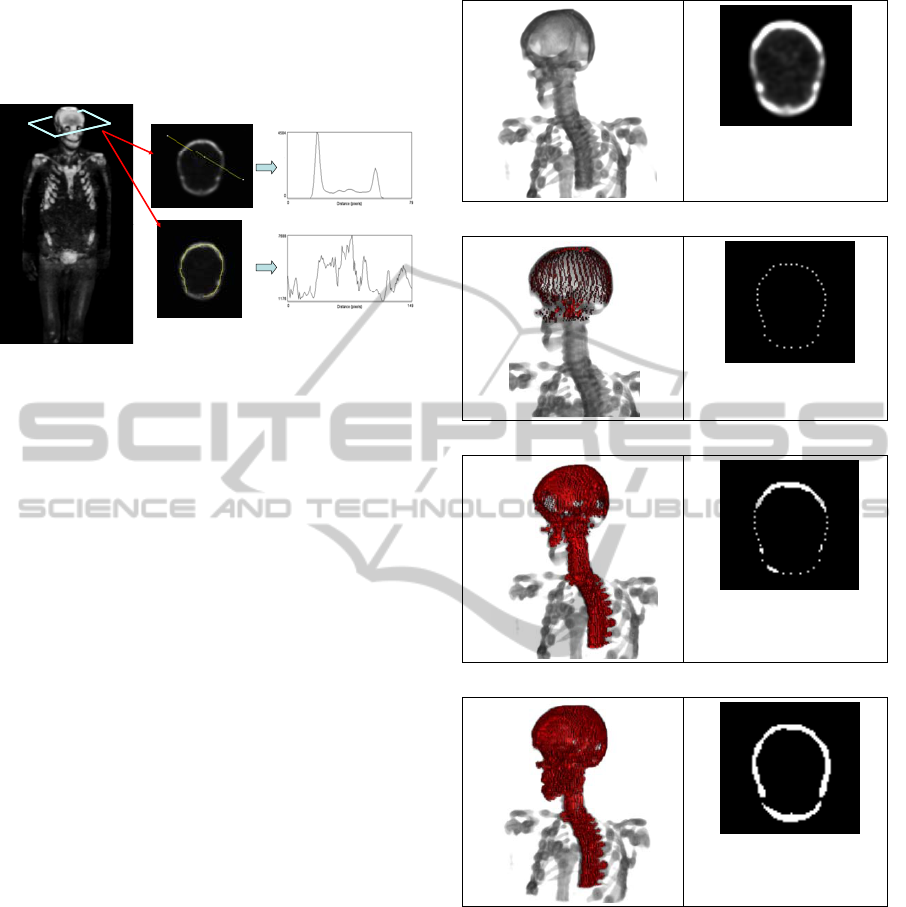
Figure 4a displays an example of a whole body
[
18
F]fluoride ion PET study, obtained with a
standard protocol of [
18
F]fluoride ion PET
acquisition described in (Grenier et al., 2005). The
dimensions of the volume are 128x128x349 pixels
and the grey levels are coded in short format (16
bits). The intensity values are proportional to the
tracer uptake.
Through the plots of two profiles, Figure 4d and
Figure 4e highlight the high variations of the
intensity and the strong inhomogeneity of the tracer
uptake due to bone metabolism. The yellow line and
curve used for the profiles were drawn on the same
slice located in the skull (Figure 4b and Figure 4c).
4.1.2 Results
In this application, the aim is to segment the skull
and the spinal column in whole body [
18
F]fluoride
ion PET studies. The adaptive region growing ARG
described in (2.3.2) was chosen to perform this
segmentation due to its ability to adapt to the local
inhomogeneity of the signal by means of its local
scale parameter.
ARG was compared to a non-adaptive region
growing method NARG, thus defined: tested voxels
are agglomerated if their grey levels belong to a
REGION GROWING: ADOLESCENCE AND ADULTHOOD - Two Visions of Region Growing: in Feature Space and
Variational Framework
293
predetermined range of variation around the mean
gray level of the evolving region. In both methods,
the initial seeds were automatically set up by a
procedure described in (Grenier et al., 2005).
Figure 4: (a) Whole body [18F]fluoride ion PET image;
(b), (c) the same slices in the skull; (d), (e) two profiles of
intensity.
Figure 5c and Figure 5d display the results of the
segmentation with NARG and ARG. For both
methods, tuning parameters were experimentally
adjusted. In the skull, ARG leads to a better
segmentation than NARG, since the evolving region
has successfully spread over the whole structure
despite the high variations of the intensities. That
demonstrates the improvements provided by the use
of the adaptive parameters.
4.2 VRG-model-based Energy:
Application to µCT Images of Mice
Kidney
VRG driven by a model-based energy (3.3.1) was
applied to segment three dimensional micro-CT
scans of mice kidney (Rose et al., 2009a). The
framework of the application is the phenotyping of
mice kidneys. The 3D reference model was obtained
by a previous manual segmentation of a reference
volume. The method was tested on a random input
volume. Slices of x-plane and y-plane are shown in
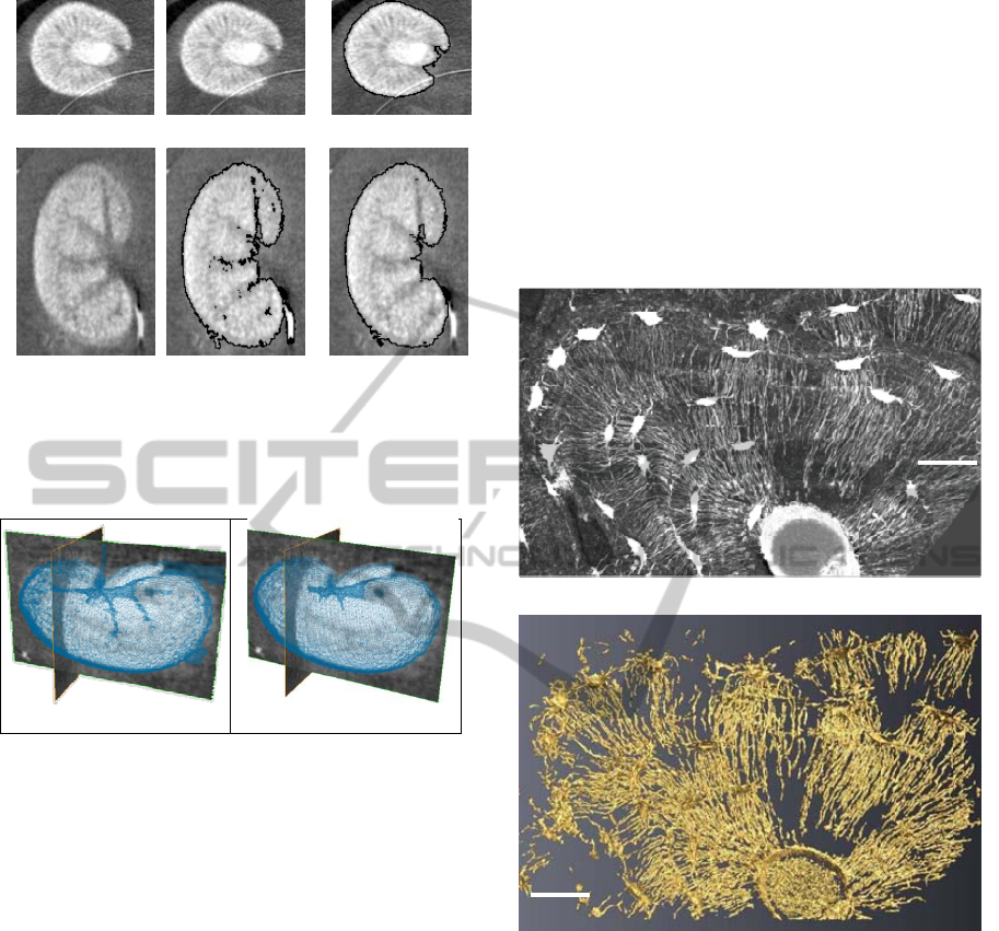
Figure 6a and Figure 6d.
We compare the results of VRG with and
without shape prior i.e using
()
T
J Φ
x
or only
()
I
J Φ
x
. Figure 6b, Figure 6e and Figure 7a show
the resulting segmentation without shape prior
()
0
α
=
. The segmentation fails to segment the
kidney due to strong inhomogeneities in the image.
Moreover, the final contour spreads through the
leaking points induced by an artifact.
Figure 6c, Figure 6f and Figure 7b illustrate
VRG results with shape prior constraint. The
(a)
(b)
(c)
(d)
Figure 5: Segmentation of [18F]fluoride ion PET image:
a) original data, b) initial seeds, c) NARG results, d) ARG
results. For each column, 3D representation is given in the
left and a slice located in the skull is given in the right.
parameter σ stepping in
()
prior
J Φ
x
was set to 1.5.
This value was not chosen too low in order to take
into account enough information about the reference
model. The hyper-parameter α was fixed to 200 and
achieves a good compromise between
(
)
prior
J
Φ
x
and
()
I
J Φ
x
since the kidney surface has been
recovered more accurately and without any leakage.
niveaux de grisniveaux de gris
0
79
0
149
(a)
(c)
(d)
(e)
(b)
VISAPP 2012 - International Conference on Computer Vision Theory and Applications
294
(a) initial image
(b) α=0 (c) α=200
(d) initial image
(e) α=0 (f) α=200
Figure 6:
μ
-CT image segmentation: (a,d) slices of the
input volume, (b, e) segmentation result without shape
prior, (c, f) segmentation result with the model-based
shape prior.
(a)
(b)
Figure 7: Segmentation results: a) without shape prior; b)
with model-based shape prior.
4.3 VRG-feature Shape Energy:
Application to SRµCT Images of
Canaliculi Network
VRG driven by a feature shape energy (3.3.2) was
applied to segment experimental data obtained with
very high resolution SR-μCT at ESRF, representing
3D images of the lacuno-canalicular structure in
human femur bone tissue. For the sample presented
in Figure 8, the acquisition resolution was 0.28µm,
the energy was set at 20.5keV and 2000 projections
were taken with a counting time of 0.8 seconds. The
osteocyte cell network is essentially composed of
ellipsoidal objects interconnected through tubular
structures. The main difficulty in segmenting this
formation arises from the slender canaliculi, the
linear features occupying only a few voxels in
diameter.
The vesselness map was created by applying
Sato’s filter on the original image. This process
enhances 3D curvilinear structures in the filtered
image. The seeds for the initialization of the region
growing were obtained by thresholding the
vesselness map. The parameters used for the
vesselness filter were determined from a previous
study based on a phantom.
Figure 8 displays the results obtained for a
800x500x100 sub-volume extracted from a (2048)
3
volume. Figure 8a shows a Maximum Intensity
Projection of the original sub-volume. Figure 8b
VRG has efficiently yielded the first segmentation
results of the canalicular system, in 3D from SR-
μCT.
(a)
(b)
Figure 8: Volume of interest showing the lacuno-
canalicular system in a human femur bone sample (image
width ~ 224 µm): a) Maximum Intensity Projection of the
original (inverted) volume; b) Isosurface of the
segmentation obtained with VRG and the feature shape
energy
()
FS
J Φ
x
.
Moreover, it has been demonstrated in a quantitative
study carried on simulated data (Pacureanu
et al.
,
2010) that VRG driven by the shape feature energy
()
FS
J
Φ
x
over performs VRG only driven by
()
I
J Φ
x
, since it can detect correct tubular
structures at a rate 20% higher and lead to better
connection of the caniculi network.
35μm
35μm
REGION GROWING: ADOLESCENCE AND ADULTHOOD - Two Visions of Region Growing: in Feature Space and
Variational Framework
295

5 CONCLUSIONS
We have presented two visions of region growing.
The first one can easily deal with multidimensional
data in the feature space and specify locally adaptive
segmentation. The second one leverages the
powerful mathematical tools of variational
framework. One major advantage is to bring
convergence properties through the minimization of
the energy functional.
Various approaches derived from both
formalisms have been successfully applied to life
imaging, yielding quite satisfying results while
enabling simple initializations, intuitive interactions
and easy understanding of tuning parameters by
users. From our knowledge, these two formalisms
should encompass whatever region growing
approaches proposed in the literature.
ACKNOWLEDGEMENTS
The authors thank the ESRF ID19 group for help
during data acquisition and Pr. M Lafage-Proust
(Inserm U890, St Etienne, France) for providing the
bones samples.
REFERENCES
Adams R, Bischof L, 1994. Seeded region growing. IEEE
Transactions on Pattern Analysis and Machine
Intelligence,
16, 641-7.
Boykov Y Y, Jolly M P, 2001. Interactive graph cuts for
optimal boundary and region segmentation of objects
in N-D images. In:
8th IEEE International Conference
on Computer Vision, Vol I, Proceedings
, 105-12.
Chan T, Zhu W, 2005. Level set based shape prior
segmentation. In:
Proceedings - 2005 IEEE Computer
Society Conference on Computer Vision and Pattern
Recognition, CVPR 2005
, 1164-70.
Chan T F, Vese L A, 2001. Active contours without edges.
IEEE Transactions on Image Processing, 10, 266-77.
Chuang C H, Lie W N, 2001. Region growing based on
extended gradient vector flow field model for multiple
objects segmentation. In:
IEEE International
Conference on Image Processing
, 74-7.
Comaniciu D, Meer P, 2002. Mean shift: A robust
approach toward feature space analysis. IEEE
Transactions on Pattern Analysis and Machine
Intelligence,
24, 603-19.
Cremers D, Sochen N, Schnörr C, 2003. Towards
recognition-based variational segmentation using
shape priors and dynamic labeling.
Scale Space
Methods in Computer Vision,
2695/2003, 388-400.
Dehmeshki J, Ye X, Costello J, 2003. Shape based region
growing using derivatives of 3D medical images:
Application to semi-automated detection of pulmonary
nodules. In: IEEE International Conference on Image
Processing
, 1085-8.
Fan J, Yau D K Y, Elmagarmid A K, Aref W G, 2001.
Automatic image segmentation by integrating color-
edge extraction and seeded region growing.
IEEE
Transactions on Image Processing,
10, 1454-66.
Foulonneau A, Charbonnier P, Heitz F, 2006. Affine-
invariant geometric shape priors for region-based
active contours.
Pattern Analysis and Machine Intelli-
gence, IEEE Transactions on,
28, 1352-7.
Frangi A F, Niessen W J, Vincken K L, Viergever M A,
1998. Multiscale vessel enhancement filtering. In:
Medical Image Computing and Computer-Assisted In-
tervention - Miccai'98
, 130-7.
Freedman D, Zhang T, 2004. Active contours for tracking
distributions. IEEE Transactions on Image
Processing,
13, 518-26.
Gastaud M, Barlaud M, Aubert G, 2004. Combining shape
prior and statistical features for active contour
segmentation.
Circuits and Systems for Video
Technology, IEEE Transactions on,
14, 726-34.
Grenier T, Revol-Muller C, Costes N, Janier M, Gimenez
G, 2005. Automated seeds location for whole body
NaF PET segmentation.
IEEE Trans. Nuc. Sci., 52,
1401-5.
Grenier T, Revol-Muller C, Costes N, Janier M, Gimenez
G, 2007. 3D robust adaptive region growing for
segmenting [18F] fluoride ion PET images. In: IEEE
Nuclear Science Symposium Conference Record
,
2644-8.
Jehan-Besson S, Barland M, Aubert G, 2003. DREAM2S:
Deformable regions driven by an Eulerian accurate
minimization method for image and video
segmentation.
International Journal of Computer
Vision,
53, 45-70.
Kass M, Witkin A, Terzopoulos D, 1987. Snakes: active
contour models. In: Proceedings - First International
Conference on Computer Vision.
, 259-68.
Lin Z, Jin J, Talbot H, 2000. Unseeded region growing for
3D image segmentation. ACM International Conferen-
ce Proceeding Series, 2000.
Malladi R, Sethian J A, Vemuri B C, 1995. Shape
modeling with front propagation: a level set approach.
IEEE Transactions on Pattern Analysis and Machine
Intelligence,
17, 158-75.
Mehnert A, Jackway P, 1997. Improved seeded region
growing algorithm.
Pattern Recognition Letters, 18,
1065-71.
Olabarriaga S D, Smeulders A W M, 2001. Interaction in
the segmentation of medical images: A survey.
Medical Image Analysis, 5, 127-42.
Pacureanu A, Revol-Muller C, Rose J L, Sanchez-Ruiz M,
Peyrin F, 2010. A Vesselness-guided Variational Se-
gmentation of Cellular Networks from 3D Micro-CT.
In: IEEE International Symposium on Biomedical Ima-
ging: From Nano to Macro
, 912 - 5.
Paragios N, Deriche R, 2002. Geodesic active regions: A
new framework to deal with frame partition problems
in computer vision.
Journal of Visual Communication
VISAPP 2012 - International Conference on Computer Vision Theory and Applications
296

and Image Representation, 13, 249-68.
Paragios N, Deriche R, 2005. Geodesic active regions and
level set methods for motion estimation and tracking.
Computer Vision and Image Understanding, 97, 259-
82.
Revol-Muller C, Peyrin F, Carrillon Y, Odet C, 2002.
Automated 3D region growing algorithm based on an
assessment function. Pattern Recognition Letters, 23,
137-50.
Revol C, Jourlin M, 1997. New minimum variance region
growing algorithm for image segmentation.
Pattern
Recognition Letters,
18, 249-58.
Rose J L, Grenier T, Revol-Muller C, Odet C, 2010.
Unifying variational approach and region growing
segmentation. In:
18th European Signal Processing
Confernce (EUSIPCO-2010)
, 1781-5.
Rose J L, Revol-Muller C, Almajdub M, Chereul E, Odet
C, 2007. Shape Prior Integrated in an Automated 3D
Region Growing method. In:
IEEE International
Conference on Image Processing ICIP'07
, 53-6.
Rose J L, Revol-Muller C, Charpigny D, Odet C, 2009a.
Shape prior criterion based on Tchebichef moments in
variational region growing. In:
IEEE International
Conference on Image Processing ICIP'09
, 1077-80.
Rose J L, Revol-Muller C, Reichert C, Odet C, 2009b.
Variational region growing. In: VISAPP-09
International Conference on Computer Vision Theory
and Applications
, 166-71.
Rother C, Kolmogorov V, Blake A, 2004. "GrabCut" -
Interactive foreground extraction using iterated graph
cuts.
Acm Transactions on Graphics, 23, 309-14.
Sato Y, Nakajima S, Shiraga N, Atsumi H, Yoshida S,
Koller T, Gerig G, Kikinis R, 1998. Three-
Dimensional Multi-Scale Line Filter for Segmentation
and Visualization of Curvilinear Structures in Medical
Images.
Medical Image Analysis, 2, 143-68.
Silverman B W, 1986.
Density Estimation for Statistiques
and Data Analysis
vol 26 (London)
Xu C, Prince J L, 1998. Generalized gradient vector flow
external forces for active contours.
Signal Processing,
71, 131-9.
Zhu S C, Yuille A, 1996. Region competition: unifying
snakes, region growing, and Bayes/MDL for
multiband image segmentation.
IEEE Transactions on
Pattern Analysis and Machine Intelligence,
18, 884-
900.
Zucker S W, 1976. Region growing: Childhood and
adolescence.
Computer Graphics and Image
Processing,
5, 382-99.
REGION GROWING: ADOLESCENCE AND ADULTHOOD - Two Visions of Region Growing: in Feature Space and
Variational Framework
297
