Nonparametric Identification of Nonlinearity
in Wiener-Hammerstein Systems
Grzegorz Mzyk
Institute of Computer Engineering, Control and Robotics, Wroclaw University of Technology,
Wybrzeze Wyspianskiego 27, 50-370 Wroclaw, Poland
Keywords: System Identification, Wiener-Hammerstein System, Nonparametric Methods, Kernel Estimate,
Convergence Analysis.
Abstract: In the paper we recover the static characteristic of Wiener-Hammerstein (sandwich) system from input-
output data. The system is excited and disturbed by random processes with arbitrary distribution. Two
kernel-based estimates are proposed and compared. It is shown that they can successfully recover the
system characteristic under small amount of a priori information about the static characteristic and the
surrounding dynamic blocks. The identified nonlinear function is not parametrized and is not assumed to be
invertible, which is common restriction in the literature. The orders of linear dynamic blocks are also
unknown. The convergence of the estimates take place for the points in which the input probability density
function in positive. The effectiveness of the algorithms is illustrated in simulation example.
1 INTRODUCTION
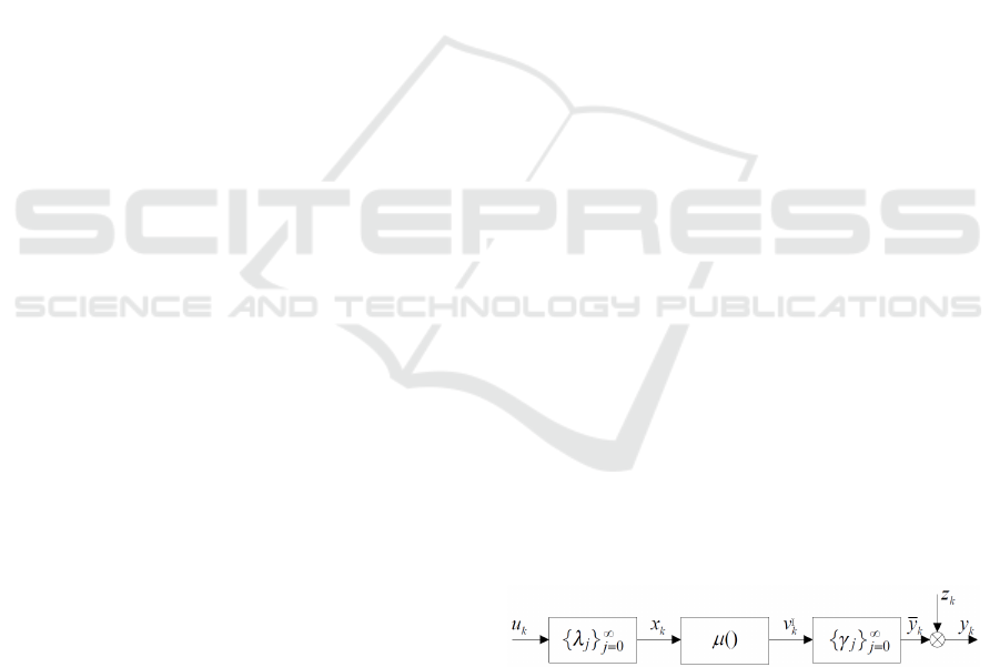
The paper addresses the problem of nonlinearity
recovering in block-oriented system of the Wiener-
Hammerstein structure (see Fig. 1). It consists of one
static nonlinear block with the characteristic
()
μ
,
surrounded by two linear dynamic components with
the impulse responses
∞
=0
}{
jj
λ
and
∞
=0
}{
jj
γ
,
respectively. Such a structure, and its particular
cases (Wiener systems and Hammerstein systems),
are widely considered in the literature because of
numerous potential applications in various domains
of science and technology (see e.g. (Giannakis and
Serpedin, 2001)). The Wiener and Wiener-
Hammerstein models allow for a good
approximation of many real processes ((Celka, et al.,
2001), (Hunter and Korenberg, 1986), (Vanbeylen,
et al., 2009), (Vörös, 2007), (Westwick and
Verhaegen, 1996)). Nevertheless, serious difficulties
in theoretical analysis force the authors to consider
only special cases, and to take restrictive
assumptions on the input signal, impulse response
and the shape of the nonlinear characteristic. In
particular, it is commonly assumed that (see e.g.
(Billings and Fakhouri, 1977), (Greblicki, 1992)-
(Greblicki and Pawlak, 2008), (Pawlak, et al., 2007),
(Bai and Rayland, 2008), (Bershad, et al., 2000),
(Lacy and Bernstein, 2003), (Wigren, 1994)): (i) the
input is a random Gaussian process, a sine wave, or
a binary signal, (ii) the static nonlinear block is
invertible, (iii) the linear dynamic blocks have finite
memory (FIR), and/or, (iv) the parametric
representation of subsystems is given a priori.
Figure 1: Wiener-Hammerstein (sandwich) system.
It was noticed in the paper that the nonparametric
algorithms proposed in (Greblicki, 2010) and
(Mzyk, 2010b) for a Wiener system, can be adopted,
without any modification, for a broad class of
Wiener-Hammerstein (sandwich) systems. All the
assumptions taken therein remain the same. Both
algorithms work under poor prior knowledge of
subsystems and excitations. We emphasize that in
contrast to earlier papers concerning sandwich and
Wiener system identification:
• the input sequence need not to be a Gaussian
white noise,
• the nonlinear characteristic is not assumed to
be invertible,
• the IIR linear dynamic blocks are admitted,
439
Mzyk G..
Nonparametric Identification of Nonlinearity in Wiener-Hammerstein Systems.
DOI: 10.5220/0003989304390445
In Proceedings of the 9th International Conference on Informatics in Control, Automation and Robotics (ICINCO-2012), pages 439-445
ISBN: 978-989-8565-21-1
Copyright
c
2012 SCITEPRESS (Science and Technology Publications, Lda.)

• the algorithm is of nonparametric nature (see
e.g. (Greblicki and Pawlak, 2008)), i.e. it is not
assumed that the subsystems can be described
with the use of finite and known number of
parameters. In consequence, the estimates are
free of the possible approximation error, or this
error can be made arbitrarily small by proper
selection of tuning parameters.
In Section 2, the problem is formulated in detail and
the assumptions imposed on signals and system
components are discussed. Then, in Section 3 we
present two nonparametric kernel-based estimates of
the nonlinearity, and analyse their properties.
Finally, in Section 4, we illustrate their behaviour in
simulation example, for various numbers of
observations and values of tuning parameters.
2 ASSUMPTIONS
We consider a tandem three-element connection
shown in Fig. 1, where
k
u
and
k
y
is a measurable
system input and output at time
k
respectively,
k
z
is a random noise,
()
μ
is the unknown characteristic
of the static nonlinearity and
∞
=0
}{
jj
λ
,
∞
=0
}{
jj
γ
- the
unknown impulse responses of the linear dynamic
components. By assumption, the interaction signals
k
x
and
k
v
are not available for measurements.
The system is described as follows
kjkj
j
k
zvy +=
−
∞
=
∑
γ
0
,
⎟
⎟
⎠
⎞
⎜
⎜
⎝
⎛
=
−
∞
=
∑
jkj
j
k
uv
λμ
0
(1)
We assume that:
(A1) The input
}{
k
u
is an i.i.d., bounded (
max
uu
k
<
; unknown
∞
<
max
u
) random process, and
there exists a probability density of the input, say
)(
ku
u
ϑ
, which is a continuous and strictly positive
function around the estimation point
x
, i.e.,
0)( >≥
ε
ϑ
x
u
.
(A2) The unknown impulse responses
∞
=0
}{
jj
λ
and
∞
=0
}{
jj
γ
of the linear IIR filters are exponentially
upper bounded, that is
, ,
11
j
j
j
j
cc
λγλλ
≤≤
(2)
some unknown
1
c
,where
10 <<
λ
is an a priori
known constant.
(A3) The nonlinear characteristic
)(x
μ
is a
Lipschitz function, i.e., it exists a positive constant
∞<l , such that for each
Rxx
ba
∈,
it holds that
.)()(
baba
xxlxx −≤−
μμ
(A4) The output noise
}{
k
z
is a zero-mean
stationary and ergodic process, which is independent
of the input
}{
k
u
.
(A5) For simplicity of presentation we also let
1
0
=
∑
=
∞
=
j
j
L
λ
,
1
0
=
∑
=
∞
=
j
j
G
γ
, and
2
1
max
=u
.
The goal is to estimate the unknown
characteristic of the nonlinearity
)(x
μ
on the
interval
),(
maxmax
uux
−
∈
on the basis of
N
input-
output measurements
N
kkk
yu
1
)},{(
=
of the whole
Wiener-Hammerstein system.
From (A1) and (A2) it holds that
∞<<
max
xx
k
,
where
j
j
ux
λ
∑
=
∞
=0
maxmax
.
Assumption (A5) is of technical meaning only.
We note that the members of the family of Wiener
systems composed by series connection of linear
filters with the impulse responses
∞
=
=
0
}{}{
2
j
c
j
j
λ
λ
and
the nonlinearities
)()(
2
xcx
μμ
=
are, for
0
2
≠
c
,
indistinguishable from the input-output point of
view. In consequence, from the input-output
viewpoint,
()
μ
can be recovered in general only up
to some domain scaling factor
2
c
, independently of
the applied identification method.
We emphasize, that in (A2), we do not assume
parametric knowledge of the linear dynamics. In
fact, the condition (rlambdaup), with unknown
1
c
, is
rather not restrictive, and characterizes the class of
stable objects. Moreover, observe that, in particular
case of FIR linear dynamics, Assumption (A2) is
fulfilled for arbitrarily small
0>
λ
.
3 THE ALGORITHMS
In the paper we propose and compare the following
two nonparametric kernel-based estimates of the
nonlinear characteristic
()
μ
∑
∑
∑
∑
=
=
−
=
=
−
⎟
⎟
⎠
⎞
⎜
⎜
⎝
⎛
−
⎟
⎟
⎠
⎞
⎜
⎜
⎝
⎛
−
=
N
k
k
j
j
jk
N
k
k
j
j
jk
k
N
Nh
xu
K
Nh
xu
Ky
x
1
0
1
0
)1(
)(
)(
)(
ˆ
λ
λ
μ
(3)
ICINCO2012-9thInternationalConferenceonInformaticsinControl,AutomationandRobotics
440

∑
∏
∑
∏
=
=
−
=
=
−
⎟
⎟
⎠
⎞
⎜
⎜
⎝
⎛
−
⎟
⎟
⎠
⎞
⎜
⎜
⎝
⎛
−
=
N
k
p
i
jk
N
k
p
i
jk
k
N
Nh
xu
K
Nh
xu
Ky
x
1
0
1
0
)2(
)(
)(
)(
ˆ
μ
(4)
In (3) and (4)
()K
is a bounded kernel function
with compact support, i.e., it fulfills the following
conditions
1)( =
∫
∞
∞−
dxxK
∞<)(sup xK
x
(5)
. some ,for 0)(
00
∞<>= xxxxK
The sequence
)(Nh
(bandwidth parameter) is such
that
. as ,0)( ∞→→ NNh
The following theorem holds.
Theorem 1. If
)(log)()( NdNdNh
λ
=
, where
)(
)(
N
NNd
γ
−
=
, and
()
w
NN
−
=
λ
γ
/1
log)( , then for
each
()
1,
2
1
∈w
the estimate (3) is consistent in the
mean square sense, i.e., it holds that
()
.0)()(
ˆ
lim
2
)1(
=−
∞→
xxE
NN
μμ
(6)
Proof. Let
x
be a chosen estimation point of
)(⋅
μ
. For a given
x
let us define a weighted
distance between the measurements
121
,...,,, uuuu
kkk −−
and
x
as
,...
)(
1
1
1
1
0
1
0
−
−
−
−
=
−++−+
+−=−=
∑
k
k
k
j
jk
k
j
k
xuxu
xuxux
λλ
λλδ
(7)
i.e.
xux −=
11
)(
δ
,
λδ
xuxux −+−=
122
)(
,
2
1233
)(
λλδ
xuxuxux −+−+−=
, etc., which can
be computed recursively as follows
.)()(
1
xuxx
kkk
−+=
−
λδδ
(8)
Making use of assumptions (A5) and (A2) we obtain
.)(
1
)( xxxx
k
k
kk
Δ=
−
+≤−
λ
λ
δ
(9)
Observe that if in turn
,)()( Nhx
k
≤Δ
(10)
then the true (but unknown) interaction input
k
x
is
located close to
x
, provided that
)(Nh
(further, a
calibration parameter) is small. If, for each
∞= ,...,1,0j
and some 0>d , it holds that
,
j
jk
d
xu
λ
≤−
−
(11)
then
.
1
1
log
λ
λ
−
+≤− dddxx
k
(12)
The condition (12) is fulfilled with probability
1 for
each
0
jj >
, where
⎣
⎦
dj
λ
log
0
=
is the solution of
the following inequality
.12
max
=≥ u
d
j
λ
On the basis of assumption
(A2), analogously as in
(9), we obtain that
,
1
1
1
0
1
0
0
0
⎟
⎠
⎞
⎜
⎝
⎛
−
++=
−
+≤−
+
=
∑
λ
λ
λ
λ
λ
λ
jd
d
xx
j
j
j
j
j
k
which yields (12). For the Wiener-Hammerstein
(sandwich) system we have
xulxy
iki
i
k
−≤−
−
∞
=
∑
χμ
0
)(
(13)
where the sequence
{
}
∞
=0i
i
χ
obviously fulfills the
condition
i
i
λχ
≤
. Let us denote the probability of
selection as
(
)
)()()( NhxPNp
k
≤
Δ
=
. To prove (6)
it suffices to show that (see (19) and (22) in (Mzyk,
2007))
0)( →Nh
(14)
,)( ∞→NNp
(15)
as
∞
→N
. The conditions (14) and (15) assure
vanishing of the bias and variance, respectively.
Since under assumptions of Theorem 3
,0)(0)( →⇒→ NhNd
(16)
in view of (12), the bias-condition (14) is obvious.
For the variance-condition (15) we have
.)()(
2
1
2
1
log)(log ++
⋅≤
ε
λλ
ε
Nd
NdNp
(17)
By inserting
NN
N
NNd
λ
γ
γ
λ
/1
log)(
)(
)/1()(
−
−
==
to (17)
we obtain
(
)
.)(
2
1
/1
2
1
loglog)()(1 ++−
⋅=⋅
εγγ
λλ
ε
NNN
NNpN
(18)
For
(
)
w
NN
−
=
λ
γ
/1
log)( and
()
1,
2
1
∈w
from (18) we
simply conclude (15) and consequently (6).
In contrast to
)(
ˆ
)1(
x
N
μ
, the estimate
)(
ˆ
)2(
x
N
μ
uses
the FIR(
p
) approximation of the linear subsystems.
We will show that since the linear blocks are
asymptotically stable, the approximation of
()
μ
can
NonparametricIdentificationofNonlinearityinWiener-HammersteinSystems
441
be made with arbitrary accuracy, i.e., by selecting
p
large enough. Let us introduce the following
regression-based approximation of the true
characteristic
()
μ
}...|{)(
121
xuuuyExm
pkkkkp
==
=
==
+−−
(19)
and the constants
. ,
1
0
1
0
j
p
j
pi
p
i
p
lg
λγ
∑∑
−
=
−
=
==
The following theorem holds.
Theorem 2. If K() satisfy (5) then it holds that
)()(
ˆ
)2(
xlmx
ppN
→
μ
(20)
in probability, as
∞
→N
, at every point
x
, for
which
0)( >x
u
ϑ
provided that
. as ,)(
2
∞→∞→ NNNh
p
Proof. The proof is a consequence of (13) and
the proof of Theorem 1 in (Greblicki, 2010).
From (19) we obtain that
=)(xm
p
⎭
⎬
⎫
⎩
⎨
⎧
===+=
+−−
−
=
∑
xuuxE
pkkiki
p
i
12
1
0
...|)(
ςμγ
where
)(
iki
pi
x
−
∞
=
∑
=
μγς
. Moreover, since
ξλ
+
∑
=
−
−
=
jkj
p
j
k
ux
1
0
, where
jkj
pj
u
−
∞
=
∑
=
λξ
it holds
that
=− )()( xlxlm
ppp
μ
{}
≤−++ )()( xlxlgE
ppp
μςξμ
{}
≤−++≤ )()( xlxlgE
ppp
μςξμ
()
,)(1
kkp
xElEug
μ
+−≤
and under stability of linear components (see
(A2)
and
(A5)) we have
.1 some ,1
00
<≤− ccg
p
p
Consequently,
ppN
xlx
εμμ
+→ )()(
ˆ
)2(
in probability, as
∞→N
, where
()
)(
maxmax0
xvluc
p
p
φε
+=
, and
1)( ≤x
φ
. Since
1lim =
∞→ pp
l
, and
0lim =
∞→ pp
ε
we conclude that
(20) is constructive in the sense that the
approximation model of
()
μ
can have arbitrary
accuracy by proper selection of
p
.
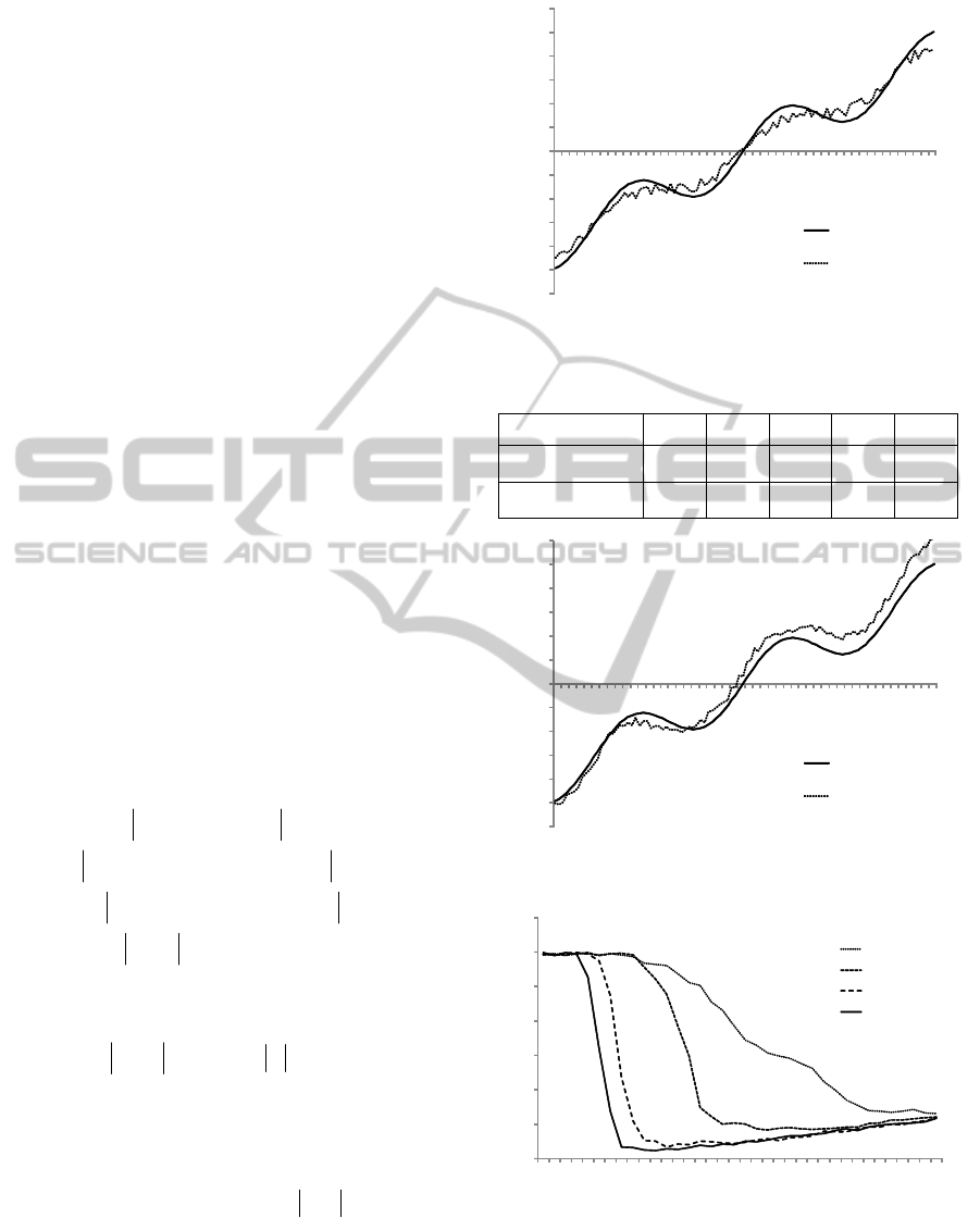
Figure 2: The true characteristic and its estimate
)(
ˆ
)1(
x
N
μ
.
Table 1: The errors of the estimates (3) and (4) versus N.
N
2
10
3
10
4
10
5
10
6
10
(
)
)(
ˆ
)1(
xERR
N
μ
6.1 4.9 0.8 0.5 0.3
(
)
)(
ˆ
)2(
xERR
N
μ
9.8 8.1 4.4 1.1 0.8
Figure 3: The true characteristic and its estimate
)(
ˆ
)2(
x
N
μ
.
Figure 4: The estimation error
))(
ˆ
(
)1(
xERR
N
μ
versus h.
‐1,20
‐1,00
‐0,80
‐0,60
‐0,40
‐0,20
0,00
0,20
0,40
0,60
0,80
1,00
1,20
‐0,78 ‐0,46 ‐0,14 0,18 0,50
truecharacteristic
estimate
‐1,20
‐1,00
‐0,80
‐0,60
‐0,40
‐0,20
0,00
0,20
0,40
0,60
0,80
1,00
1,20
‐0,78 ‐0,46 ‐0,14 0,18 0,50
truecharacteristic
estimate
0,00
1,00
2,00
3,00
4,00
5,00
6,00
7,00
0,00 0,20 0,40 0,60
N=100
N=1000
N=10000
N=100000
ICINCO2012-9thInternationalConferenceonInformaticsinControl,AutomationandRobotics
442

Figure 5: The estimation error
))(
ˆ
(
)2(
xERR
N
μ
versus h.
4 NUMERICAL EXAMPLE
In the computer experiment we generated uniformly
distributed i.i.d. input sequence
]1,1[−∼Uu
k
and the
output noise
]1.0,1.0[−∼Uz
k
. We simulated the IIR
linear dynamic subsystems
kkk
uxx 5.05.0
1
+=
−
and
k
kk
vyy 5.05.0
1
+=
−
,
i.e.
1
5.0
+
==
j
jj
γλ
,
∞= ,...,1,0j
, sandwiched with
the not invertible static nonlinear characteristic
()
xxx 10sin2.0)( +=
μ
.
The nonparametric estimates (3) and (4) were
computed on the same simulated data
N
kkk
yu
1
)},{(
=
.
In
(A2) we assumed
8.0=
λ
and in (19) we took
3=p
. The estimation error was computed
according to the rule
()( )
∑
=
−=
0
1
2
)()(
)()(
ˆ
)(
ˆ
N
i
ii
NN
xxxERR
μμμ
(21)
where
0
1
)(
}{
N
i
i
x
=
is the grid of equidistant estimation
points. The result of estimation for
1000=N
are
shown in Fig. 2 and Fig. 3. The routine was repeated
for various values of the tuning parameter
h . As can
be seen in Fig. 4 and Fig. 5, according to intuition,
improper selection of
h increases the variance or
bias of the estimate. Table 1 shows the errors (21) of
)(
ˆ
)1(
x
N
μ
and
)(
ˆ
)2(
x
N
μ
. It illustrates advantages of
)(
ˆ
)1(
x
N
μ
over
)(
ˆ
)2(
x
N
μ
, when the number of
measurements tends to infinity and the linear
component in the Wiener system has infinite
impulse response (IIR). The bandwidth parameters
was set according to
() ()
ww
NN
NNNh
−−
−−
=
λλ
λ
/1/1
loglog
log)(
with
75.0=w
in
(3), and
)12/(1
)(
+−
=
p
NNh
with
5=p
in (4).
5 FINAL REMARKS
In the paper, the nonlinear characteristic of Wiener-
Hammerstein system is successfully recovered from
the input-output data under small amount of a priori
information. The estimates work under IIR dynamic
blocks, non-Gaussian input and for non-invertible
characteristics. Since the Hammerstein systems and
the Wiener systems are special cases of the
sandwich system, considered in the paper, the
proposed approach is universal in the sense that it
can be applied without the prior knowledge of the
system structure.
As regards the limit properties, the estimates
)(
ˆ
)1(
x
N
μ
and
)(
ˆ
)2(
x
N
μ
are not equivalent. First of them
has slower rate of convergence (logarithmic), but it
converges to the true system characteristic, since the
model becomes more complex as the number of
observations tends to infinity. The main limitation is
assumed knowledge of
λ
, i.e., the upper bound of
the impulse response. On the other hand the
convergence of the estimate
)(
ˆ
)2(
x
N
μ
is faster
(polynomial), but the estimate is biased, even
asymptotically. However, the bias can be made
arbitrarily small by selecting the cut-off parameter
p
large enough.
As it was shown in (Hasiewicz and Mzyk, 2009),
the nonparametric methods allow for decomposition
of the identification task of block-oriented system
and can support estimation of its parameters.
Computing of both estimates
)(
ˆ
)1(
x
N
μ
,
)(
ˆ
)2(
x
N
μ
and
the distance
)(x
k
δ
has the numerical complexity
)(NO
, and can be performed in recursive or semi-
recursive version (see (Greblicki and Pawlak,
2008)).
The principal question in Wiener-Hammerstein
system identification problem is selection of
adequate method. The scope of application of each
estimate is limited by a specific set of associated
assumptions. Most of them requires a priori known
parametric type of model, Gaussian input, FIR
dynamics or invertible characteristic. Since the
general Wiener-Hammerstein system identification
problem includes many difficult aspects, existence
of one universal algorithm cannot be expected. In
the light of this, the nonparametric approach seems
0,00
2,00
4,00
6,00
8,00
10,00
12,00
0,0 0 0,2 0 0,40 0,60
N=100
N=1000
N=10000
N=100000
NonparametricIdentificationofNonlinearityinWiener-HammersteinSystems
443

to be good tool, which allows for combining selected
methods (see e.g. (Mzyk, 2010b)), depending on
specificity of the particular task. Moreover, pure
nonparametric estimates are the only possible
choice, when the prior knowledge of the system is
poor or uncertain.
Nonparametric approach offers simple
algorithms, which are asymptotically free of
approximation error, i.e. they converge to the true
system characteristics. However, the purely
nonparametric methods are not commonly exploited
in practice for the following reasons: (i) they depend
on various tuning parameters and functions; in
particular, proper selection of kernel and the
bandwidth parameter or orthonormal basis and the
scale factor are critical for the obtained results, (ii)
the prior knowledge of subsystems is completely
neglected; the estimates are based on measurements
only, and the resulting model may be not satisfactory
when the number of measurements is small, and (iii)
bulk number of estimates must be computed when
the model complexity grows large.
REFERENCES
Bai, E. W., Reyland, J., 2008. Towards identification of
Wiener systems with the least amount of a priori
information on the nonlinearity. Automatica. Vol. 44,
No. 4, pp. 910-919.
Bai, E. W., 2003. Frequency domain identification of
Wiener models. Automatica. Vol. 39, No. 9, pp. 1521-
-1530.
Bershad, N. J., Celka, P., Vesin, J. M, 2000. Analysis of
stochastic gradient tracking of time-varying
polynomial Wiener systems. IEEE Transactions on
Signal Processing. Vol. 48, No. 6, pp. 1676-1686.
Billings, S. A., Fakhouri, S. Y., 1977. Identification of
nonlinear systems using the Wiener model.
Automatica. Vol. 13, No. 17, pp. 502-504.
Boutayeb, M., Darouach, M., 1995. Recursive
identification method for MISO Wiener-Hammerstein
Model. IEEE Transactions on Automatic Control. Vol.
40, No. 2, pp. 287-291.
Celka, P., Bershad, N. J., Vesin, J. M., 2001. Stochastic
gradient identification of polynomial Wiener systems:
analysis and application. IEEE Transactions on Signal
Processing. Vol. 49, No. 2, pp. 301-313.
Giannakis, G. B., Serpedin, E., 2001. A bibliography on
nonlinear system identification. Signal Processing.
Vol. 81, pp. 533-580.
Greblicki, W., 1992. Nonparametric identification of
Wiener systems. IEEE Transactions on Information
Theory. Vol. 38, pp. 1487-1493.
Greblicki, W., 1997. Nonparametric approach to Wiener
system identification. IEEE Transactions on Circuits
and Systems -- I: Fundamental Theory and
Applications. Vol. 44, No. 6, pp. 538-545.
Greblicki, W., 2010. Nonparametric input density-free
estimation of the nonlinearity in Wiener systems.
IEEE Transactions on Information Theory. Vol. 56,
No. 7, pp. 3575-3580.
Greblicki, W., Mzyk, G., 2009. Semiparametric approach
to Hammerstein system identification. Proceedings of
the 15th IFAC Symposium on System Identification,
pp. 1680-1685, Saint-Malo, France.
Greblicki, W., Pawlak, M, 2008. Nonparametric System
Identification, Cambridge University Press, 2008.
Hasiewicz, Z., 1987. Identification of a linear system
observed through zero-memory non-linearity.
International Journal of Systems Science. Vol. 18, pp.
1595-1607.
Hasiewicz, Z., Mzyk, G., 2004. Combined parametric-
nonparametric identification of Hammerstein systems.
IEEE Transactions on Automatic Control. Vol. 49, pp.
1370-1376.
Hasiewicz, Z., Mzyk, G., 2009. Hammerstein system
identification by non-parametric instrumental
variables. International Journal of Control. Vol. 82,
No. 3, pp. 440-455.
Hunter, I. W., Korenberg, M. J., 1986. The identification
of nonlinear biological systems: Wiener and
Hammerstein cascade models. Biological Cybernetics.
Vol. 55, pp. 135-144.
Lacy, S. L., Bernstein, D. S., 2003. Identification of FIR
Wiener systems with unknown, non-invertible,
polynomial non-linearities. International Journal of
Control
. Vol. 76, No. 15, pp. 1500-1507.
Mzyk, G., 2007. A censored sample mean approach to
nonparametric identification of nonlinearities in
Wiener systems. IEEE Transactions on Circuits and
Systems -- II: Express Briefs. Vol. 54, No. 10, pp. 897-
901.
Mzyk, G., 2009. Nonlinearity recovering in Hammerstein
system from short measurement sequence. IEEE
Signal Processing Letters. Vol. 16, No. 9, pp. 762-
765.
Mzyk, G., 2010. Parametric versus nonparametric
approach to Wiener systems identification. Lecture
Notes in Control and Information Sciences. Vol. 404,
Chapter 8.
Mzyk, G., 2010. Wiener-Hammerstein system
identification with non-gaussian input. IFAC
International Workshop on Adaptation and Learning
in Control and Signal Processing.
Nesic, D., Bastin, G., 1999. Stabilizability and dead-beat
controllers for two classes of Wiener-Hammerstein
models. IEEE Transactions on Automatic Control.
Vol. 44, No. 11, pp. 2068-2071.
Pawlak, M., Hasiewicz, Z., Wachel, P., 2007. On
nonparametric identification of Wiener systems. IEEE
Transactions on Signal Processing. Vol. 55, No. 2, pp.
482-492.
Vanbeylen, L., Pintelon, R., Schoukens, J., 2009. Blind
maximum-likelihood identification of Wiener systems.
ICINCO2012-9thInternationalConferenceonInformaticsinControl,AutomationandRobotics
444

IEEE Transactions on Signal Processing. Vol. 57, No.
8, pp. 3017-3029.
Vörös, J., 2007. Parameter identification of Wiener
systems with multisegment piecewise-linear
nonlinearities. Systems and Control Letters. Vol. 56,
pp. 99-105.
Westwick, D., Verhaegen, M., 1996. Identifying MIMO
Wiener systems using subspace model identification
methods. Signal Processing. Vol. 52, pp. 235-258.
Wiener, N, 1958. Nonlinear Problems in Random Theory.
Wiley, New York.
Wigren, T., 1994. Convergence analysis of recursive
identification algorithms based on the nonlinear
Wiener model, IEEE Transactions on Automatic
Control. Vol. 39, pp. 2191-2206.
NonparametricIdentificationofNonlinearityinWiener-HammersteinSystems
445
