
Spacecrafts' Control Systems Effective Variants Choice
with Self-Configuring Genetic Algorithm
Eugene Semenkin and Maria Semenkina
Institute of Computer Sciences and Telecommunication, Siberian State Aerospace University,
Krasnoyarskiy Rabochiy Ave., 31, 660014, Krasnoyarsk, Russia
Keywords: Spacecraft Control System, Control Contours Models, Markov Chains, Effective Variant Choice,
Optimization, Self-configuring Genetic Algorithm.
Abstract: The work of the spacecraft control system is modeled with Markov chains. Small and large models for the
technological and command-programming control contours are developed. The way of the calculation of the
control contour effectiveness indicators is described. Special self-configuring genetic algorithm that requires
no settings determination and parameter tuning is proposed for choosing effective variants of spacecraft
control system. The high performance of the suggested algorithm is demonstrated through experiments with
test problems and then is validated by the solving hard optimization problems.
1 INTRODUCTION
Current efforts by the developers of spacecraft are
concentrated upon increasing the usage effectiveness
of existing spacecraft systems and improving the
development and design process for new ones. One
of the ways to achieve these aims is a rational choice
of the effective variants of the developing systems.
This requires the application of adequate models,
effective algorithmic tools and powerful computers.
This application will allow multivariant analysis of
the developing systems that is currently not so easy
due to their complexity.
One of the most difficult and underdeveloped
problems is that of the synthesis of a spacecraft's
control systems. These are currently solved with
more empirical methods rather than formalized
mathematical tools. Usually, the spacecraft control
system design is a sophisticated process involving
the cooperation of numerous experts and
departments each having their own objectives and
constraints. Nevertheless, it is possible to
mathematically model some subproblems and to
obtain some qualitative results of computations and
tendencies that could provide interesting information
for experts. The usual position of system analyst in
such a situation is as mediator for high level decision
making, dealing with informal problems for which it
is impossible to develop a mathematical model, and
lower level computations for which strong
mathematical models exist but the results of them do
not always match. If, in this intermediate position
when mathematical models are strong enough but
very complicated for analysis, we intend to
implement a decision support system for the choice
of effective variants then we have to realize that the
optimization problems arise here are intractable for
the majority of known algorithms.
We suggest modeling the functioning process of
a spacecraft's control subsystems with Markov
chains. We explain the modeling with small models
and then give illustration of large models that are
closer to real system. The problem of choosing an
effective variant for a spacecraft's control system is
formulated as a multi-scale optimization problem
with algorithmically given functions. In this paper,
we use self-configuring genetic algorithm to solve
the optimization problem.
The rest of the paper is organized in the following
way. Section 2 briefly describes the modeled system.
In Sections 3 and 4 we describe small size models for
two control contours. Section 5 illustrates briefly the
view of large models. In Section 6 we describe the
proposed optimization algorithm and in Section 7 we
evaluate its performance on the test problems. In
Section 8, the results of the algorithm performance
evaluation on spacecraft control system optimization
problems is given, and in the Conclusion section the
article content is summarized and future research
directions are discussed.
84
Semenkin E. and Semenkina M..
Spacecrafts’ Control Systems Effective Variants Choice with Self-configuring Genetic Algorithm .
DOI: 10.5220/0004042200840093
In Proceedings of the 9th International Conference on Informatics in Control, Automation and Robotics (ICINCO-2012), pages 84-93
ISBN: 978-989-8565-21-1
Copyright
c
2012 SCITEPRESS (Science and Technology Publications, Lda.)

2 PROBLEM DESCRIPTION
The system for monitoring and control of an orbital
group of telecommunication satellites is an
automated, distributed, information-controlling
system that includes in its composition on-board
control complexes (BCC) of spacecrafts; telemetry,
command and ranging (TSR) stations; data
telecommunication subsystems; and a mission
control center (MCC). The last three subsystems are
united in the ground-based control complex (GCC).
GCC interacts with BCC(s) through a distributed
system of TCR stations and data telecommunication
systems that include communication nodes in each
TCR, channels and MCC's associated
communication equipment. BCC is the controlling
subsystem of the spacecraft that ensures real time
checking and controlling of on-board systems
including pay-load equipment (PLE) as well as
fulfilling program-temporal control. Additionally,
BCC ensures the interactivity with ground-based
tools of control. The control functions fulfilled by
subsystems of the automated control system are
considered to form subsets called "control contours"
that contain essentially different control tasks.
Usually, one can consider the technological control
contour, command-programming contour, purpose
contour, etc.
Each contour has its own indexes of control
quality that cannot be expressed as a function of
others. This results in many challenges when
attempting to choose an effective control system
variant to ensure high control quality with respect to
all of the control contours. A multicriterial
optimization problem statement is not the only
problem. For most of the control contours, criterion
cannot be given in the form of an analytical function
of its variables but exists in an algorithmic form
which requires a computation or simulation model to
be run for criterion evaluation at any point.
In order to have the possibility of choosing an
effective variant of such a control system, we have
to model the work of all control contours and then
combine the results in one optimization problem
with many models, criteria, constraints and
algorithmically given functions of mixed variables.
We suggest using evolutionary algorithms (EAs) to
solve such optimization problems as these
algorithms are known as good optimizers having no
difficulties with the described problem properties
such as mixed variables and algorithmically given
functions. To deal successfully with many criteria
and constraints we just have to incorporate
techniques, well known in the EA community.
However, there is one significant obstacle in the use
of EAs for complicated real world problems. The
performance of EAs is essentially determined by
their settings and parameters which require time and
computationally consuming efforts to find the most
appropriate ones.
To support the choice of effective variants of
spacecrafts' control systems, we have to develop the
necessary models and resolve the problem of EAs
settings.
3 TECHNOLOGICAL CONTROL
CONTOUR MODELING
The main task of the technological control contour is
to provide workability of the spacecraft for the
fulfillment of its purposes, i.e., the detecting and
locating of possible failures and malfunctions of the
control system and pay-load and restoring their lost
workability by the activation of corresponding
software and hardware tools. The basic index of the
quality for this contour is the so called readiness
coefficient, i.e., a probability to be ready for work
(hasn’t malfunctioned) at each point in time.
We consider simplified control system to
describe our modeling approach. Let the system
consist of three subsystems: on-board pay-load
equipment, on-board control complex and ground-
based control complex. Let us assume that GCC
subsystems are absolutely reliable but PLE and BCC
can fail. If PLE failed, BCC can restore it using its
own software tools with the probability p
0
or,
otherwise, re-directs restoring process (with the
probability 1-p
0
) into GCC that finishes restoring
with the probability equal to 1. In the case of a BCC
malfunction, GCC restores it with the probability
equal to one.
We can use a Markov chain approach to model a
spacecraft’s’ control system operation because of its
internal features such as high reliability and work
stability, e.g., two simultaneous failures are almost
impossible, there is no aftereffect if malfunction
restoring is finished, etc. That is why we will
suppose that all stochastic flows in the system are
Poisson ones with corresponding intensities:
1
is an
intensity of PLE malfunctions,
2
is an intensity of
BCC malfunctions,
1
is an intensity of PLE
restoring with BCC,
2
is an intensity of PLE
restoring with GCC,
3
is an intensity of BCC
restoring with GCC.
In the described situation, there are five possible
states of the system:
Spacecrafts' Control Systems Effective Variants Choice with Self-configuring Genetic Algorithm
85
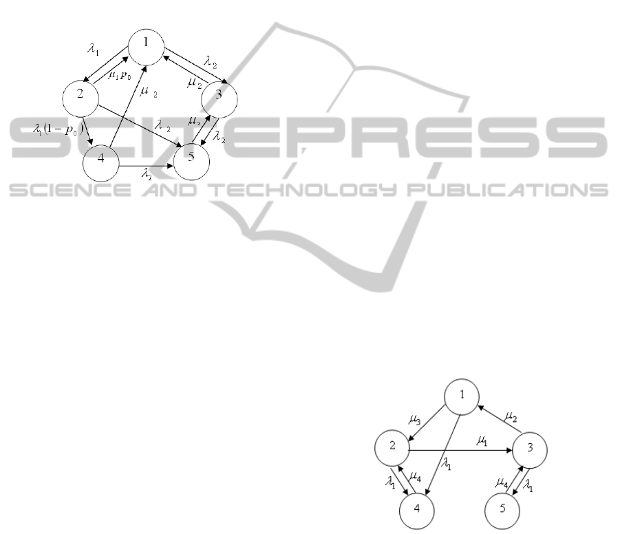
1. All subsystems are workable.
2. PLE malfunction, BCC is restoring PLE, GCC is
free.
3. BCC malfunction, GCC is restoring BCC, PLE is
workable.
4. PLE malfunction, BCC is workable and free,
GCC is recovering PLE.
5. PLE malfunction, BCC malfunction, GCC is
recovering PLE, and BCC is waiting for
recovering.
States graph can be drawn as is shown in Figure 1.
Figure 1: States graph of Markov chain for the simplified
model of a technological control contour.
Corresponding Kolmogorov's equation system is:
P
1
·(
1
+
2
) -
1
·p
0
·P
2
-
3
·P
3
-
2
·P
4
= 0,
P
2
·(
1
+
2
) -
1
·P
1
= 0,
P
3
·(
1
+
3
) -
2
·P
1
-
2
·P
5
= 0,
P
4
·(
2
+
2
) - (1-p
0
)·
1
·P
2
= 0,
P
5
·
2
-
2
·P
2
-
1
·P
3
-
2
·P
4
= 0,
P
1
+ P
2
+ P
3
+ P
4
+ P
5
= 1.
The last equation is needed for normalization and
should replace any of previous ones.
Given final probabilities that the system remains
in the corresponding state, as the solution of this
equation system, the control quality indicators, i.e.,
readiness coefficients, can be calculated in following
way:
1. Spacecraft readiness coefficient k
s
= P
1
.
2. PLE readiness coefficient k
PLE
= P
1
+ P
3
.
3. BCC readiness coefficient k
BCC
= P
1
+ P
2
+ P
4
.
To have the effective variant of the spacecraft
control system we have to maximize the readiness
coefficients subject to constraints on the on-board
computer memory and computational efforts needed
for the technological contour functions realization.
Optimization variables are stochastic flow intensities
1
,
2
,
1
,
2
,
3
, as well as p
0
, i.e., the distribution
of contour functions between BCC and GCC. If they
are characteristics of existing variants of software-
hardware equipment, we have the problem of
effective variant choice, i.e., a discrete optimization
problem. In case of a system preliminary design,
some of the intensities can be real numbers and we
will have to implement corresponding software and
hardware to ensure an optimal solution. Recall that
obtained optimization problem has algorithmically
given objective functions so before the function
value calculation we must solve the equations
system.
4 COMMAND-PROGRAMMING
CONTROL CONTOUR
MODELING
The main task of this contour is the maintenance of
the tasks of creating of the command-programming
information (CPI), transmitting it to BCC and
executing it and control action as well as the
realization of the temporal program (TP) regime of
control.
We can use Markov chains for modeling this
contour for the same reasons. If we suppose that
BCC can fail and GCC is absolutely reliable, then
we can introduce the following notations:
1
is the
intensity of BCC failures,
1
is the intensity of
temporal program computation,
2
is the intensity
CPI loading into BCC,
3
is the intensity of temporal
program execution,
4
is the intensity of BCC being
restored after its failure. The graph of the states for
command-programming contour can be drawn as in
Figure 2.
Figure 2: States graph of Markov chain for simplified
model of command-programming control contour.
There are also five possible states for this contour:
1. BCC fulfills TP, GCC is free.
2. BCC is free, GCC computes TP.
3. BCC is free; GCC computes CPI and loads TP.
4. BCC is restored with GCC which is waiting for
continuation of TP computation.
ICINCO 2012 - 9th International Conference on Informatics in Control, Automation and Robotics
86
5. BCC is restored with GCC which is waiting for
continuation of CPI computation.
BCC, restored after any failure in state 1, cannot
continue its work and has to wait for a new TP
computed with GCC. If BCC has failed in state 2 or
state 3 then GCC can continue its computation only
after BCC restoring completion.
If we assume for simplicity that all flows in the
system are Poisson ones, the system of
Kolmogorov's equations can be written as follows.
P
1
·(
1
+
3
) -
2
·P
3
= 0,
P
2
·(
1
+
1
) -
3
·P
1
-
4
·P
4
= 0,
P
3
·(
1
+
2
) -
1
·P
2
-
4
·P
5
= 0,
P
4
·
4
-
1
·P
1
-
1
·P
2
= 0,
P
5
·
4
-
1
·P
3
= 0,
P
1
+ P
2
+ P
3
+ P
4
+ P
5
= 1.
After solving the Kolmogorov's system, we can
calculate the necessary indexes of control quality for
the command-programming contour. Basic indexes
of this contour are the time interval when the
temporal program control can be fulfilled without a
change of TP, i.e., the duration of the independent
operating of the spacecraft for this contour (has to be
maximized) and the duration of BCC and GCC
interactions when loading TP for the next interval of
independent operation of the spacecraft (has to be
minimized). Mathematically these can be described
as follows:
T = P
1
/(
2
P
3
) is an average time of TP
fulfillment with BCC;
t
1
= (P
3
+ P
5
)/(
1
P
2
) – an average time of BCC
interaction with GCC when TP is loading;
t
2
= (P
2
+ P
3
+ P
4
+ P
5
)/P
1
(
1
+
3
) – an average
time from the start of TP computation till the start of
TP fulfillment by BCC.
The last indicator also has to be minimized.
All these indicators have to be optimized through
the appropriate choice of the operations intensities
that are the parameters of the software-hardware
equipment included in the control system.
Corresponding optimization problem has the same
properties as described above.
5 MODELS GENERALISATION
We described above the simplified models of two
control contours in order to demonstrate the
modeling technique. The developed models are not
adequate for the use in the spacecraft control system
design process because of the unrealistic assumption
of GCC reliability.
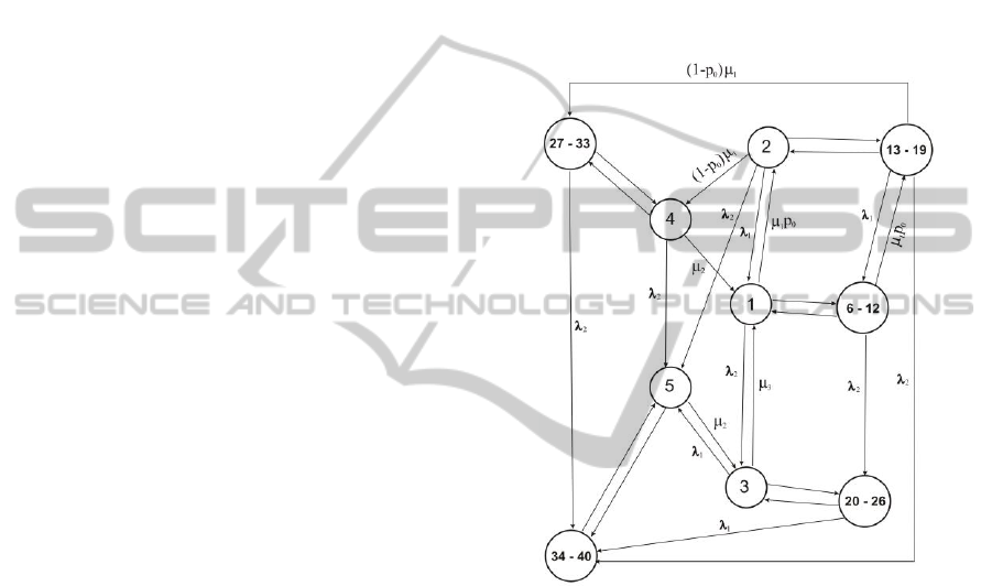
If we suppose the GCC can fail then we have to
add the states when GCC fails while the system is in
any state. Let us consider the model of the
technological control contour with an unreliable
GCC which is assumed to be a single unit without
any subsystems, i.e., we will model the whole GCC
malfunctioning if any of its subsystems fails. Figure
3 shows the corresponding states graph with 10
nodes and 27 transitions that seems simple enough
for analysis. However, five new nodes with
numeration such as 6-12 or 13-19 represent states
where at least one of GCC subsystems failed.
Figure 3: States graph of Markov chain for the model of
the technological control contour with an unreliable GCC.
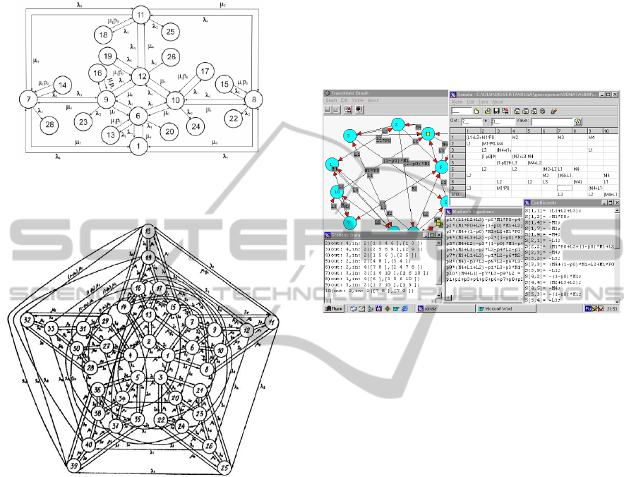
GCC in our problem description consists of three
subsystems groups – TCR stations, data
communication subsystem, and MCC equipment.
Considering all three groups as one unit, we will
have three GCC subsystems. If any of them can fail,
the new nodes and possible transitions will have a
view as it is shown in the Figure 4.
We will not describe the meaning of all notion in
details, recall that
i
indicate the intensities of
subsystems failures and
j
indicate the intensities of
subsystems being restoring by BCC (for PLE) or
GCC (for all subsystems including itself).
Not all transitions are depicted in this figure. The
whole states graph for this case consists of 40 states
and 146 transitions and is schematically depicted in
Figure 5. Corresponding Kolmogorov's equation
system contains 40 lines.
Spacecrafts' Control Systems Effective Variants Choice with Self-configuring Genetic Algorithm
87
Under the same conditions, the states graph for
the command-programming contour consists of 96
states and more than 300 transitions and cannot be
shown here.
Figure 4: States graph of Markov chain for description of
GCC failures while spacecraft remains reliable (state 1).
Figure 5: States graph of Markov chain for modeling
technological control contour with unreliable GCC
subsystems.
Going deeper into the details we must continue
dividing the subsystems groups (TCR stations,
telecommunication system, MCC) in parts. Then we
must unify models of all contours of the spacecraft
and models of identical contours of different
spacecrafts of the orbital group. Additionally, in
some cases we cannot use simple Markov chain
models and need a more sophisticated simulation
models. Certainly, this work cannot be done without
an adequate computation tool.
In the next stage of our research we have
developed and implemented a decision support
system for spacecraft control systems modeling with
stochastic processes models. This DSS suggests
questions to aerospace engineers designing
spacecraft control systems in their terms relative to
system structure, its subsystems, possible states and
transitions, executed operations, etc. Giving the
answers to these questions the DSS generates the
necessary data structure, the lists of states and
transitions with their descriptions in designer terms
and definitions, Kolmogorov's equations system, etc.
It can also depict the states graph in simple cases
when there are not too many states and transitions.
Working windows of this decision support system is
shown in Figure 6.
Figure 6: Working windows of DSS for control systems
modeling.
This DSS is able also to solve optimization
problems with some adaptive search algorithms.
As has been stressed above, optimization
problems arising in the described situation are hard
to solve. That is why we suggest here using our
modified genetic algorithm.
6 OPTIMIZATION
ALGORITHMS DESCRIPTION
Evolutionary algorithms (EA), the best known
representatives of which are genetic algorithms
(GA), are well known optimization techniques based
on the principles of natural evolution (Eiben, Smith,
2003). Although GAs are successful in solving many
real world optimization problems (Haupt, Haupt,
2004), their performance depends on the selection of
the GA settings and tuning their parameters (Eiben,
Hinterding and Michalewicz, 1999). GAs usually
use a bit-string solution representation, but other
decisions have to be made before the algorithm can
run. The design of a GA consists of the choice of
variation operators (e.g. recombination and
mutation) that will be used to generate new solutions
from the current population and the parent selection
operator (to decide which members of the population
ICINCO 2012 - 9th International Conference on Informatics in Control, Automation and Robotics
88

are to be used as inputs to the variation operators), as
well as a survival scheme (to decide how the next
generation is to be created from the current one and
outputs of the variation operators). Additionally, real
valued parameters of the chosen settings (the
probability of recombination, the level of mutation,
etc.) have to be tuned (Eiben et al., 1999).
The process of settings determination and
parameters tuning is known to be a time-consuming
and complicated task. Much research has tried to
deal with this problem. Some approaches tried to
determine appropriate settings by experimenting
over a set of well-defined functions or by theoretical
analysis. Another set of approaches, usually
applying terms like "self-adaptation" or "self-
tuning", are eliminating the setting process by
adapting settings through the algorithm execution.
There exist much research devoted to "self-
adapted" or "self-tuned" GA and authors of the
corresponding papers determine similar ideas in very
different ways, all of them aimed at reducing the
role of human expert in algorithms designing.
The main idea of the approach used in this paper
relies to automated selecting and using existing
algorithmic components. That is why our algorithms
might be called as self-configuring ones.
In order to specify our algorithms more
precisely, one can say that, according to (Angeline,
1995) classification, we use dynamic adaptation on
the level of population (Meyer-Nieberg and Beyer,
2007). The probabilities of applying the genetic
operators are changed "on the fly" through the
algorithm execution. According to the classification
given in (Gomez, 2004) we use centralized control
techniques (central learning rule) for parameter
settings with some differences from the usual
approaches. Operator rates (the probability to be
chosen for generating off-spring) are adapted
according to the relative success of the operator
during the last generation independently of the
previous results. This is why our algorithm avoids
problem of high memory consumption typical for
centralized control techniques (Gomez, 2004).
Operator rates are not included in individual
chromosome and they are not subject to the
evolutionary process. All operators can be used
during one generation for producing off-spring one
by one.
Having in mind the necessity to solve hard
optimization problems and our intention to organize
GA self-adaptation to these problems, we must first
improve the GA flexibility before it can be adapted.
For this reason we have tried to modify the most
important GA operator, i.e., crossover.
The uniform crossover operator is known as one
of the most effective crossover operators in
conventional genetic algorithm (Syswerda, 1989; De
Jong, Spears, 1991). Moreover, nearly the
beginning, it was suggested to use a parameterized
uniform crossover operator and it was shown that
tuning this parameter (the probability for a parental
gene to be included in off-spring chromosome) one
can essentially improve "The Virtues" of this
operator (De Jong and Spears, 1991). Nevertheless,
in the majority of cases using the uniform crossover
operator the mentioned possibility is not adopted and
the probability for a parental gene to be included in
off-spring chromosome is given equal to 0.5 (Eiben
and Smith, 2003; Haupt and Haupt, 2004).
Thus it seems interesting to modify the uniform
crossover operator with an intention to improve its
performance. Desiring to avoid real number
parameter tuning, we suggested introducing
selective pressure on the stage of recombination
(Semenkin and Semenkina, 2007) making the
probability of a parental gene to be taken for off-
spring dependable on parent fitness values. Like the
usual GA selection operators, fitness proportional,
rank-based and tournament-based uniform crossover
operators have been added to the conventional
operator called here the equiprobable uniform
crossover.
Although the proposed new operators, hopefully,
give higher performance than the conventional
operators, at the same time the number of algorithm
setting variants increases that complicates
algorithms adjusting for the end user. That is why
we need suggesting a way to avoid this extra effort
for the adjustment.
With this aim, we apply operators’ probabilistic
rates dynamic adaptation on the level of population
with centralized control techniques. To avoid real
parameters precise tuning, we use setting variants,
namely types of selection, crossover, population
control and a level of mutation (medium, low, high).
Each of these has its own probability distribution.
E.g., there are 5 settings of selection – fitness
proportional, rank-based, and tournament-based with
three tournament sizes. During the initialization all
probabilities are equal to 0.2 and they will be
changed according to a special rule through the
algorithm’s execution in such a way that a sum of
probabilities should be equal to 1 and no probability
could be less than a preconditioned minimum
balance. The list of crossover operators includes 11
items, i.e., 1-point, 2-point and four uniform
crossovers all with two numbers of parents (2 and
7). The "idle crossover" is included in the list of
Spacecrafts' Control Systems Effective Variants Choice with Self-configuring Genetic Algorithm
89
crossover operators to make crossover probability
less than 1 that is used in conventional algorithms to
model "childless couple".
When the algorithm has to create the next off-
spring from the current population, it firstly has to
configure settings, i.e. to form the list of operators
with the use of the probability operator distributions.
Then the algorithm selects parents with the chosen
selection operator, produces an off-spring with the
chosen crossover operator, mutates this off-spring
with the chosen mutation probability and puts it into
the intermediate population. When the intermediate
population is filled, the fitness evaluation is
executed and operator rates (the probabilities to be
chosen) are updated according to the operator
productivity. Then the next parental population is
formed with the chosen survival selection operator.
The algorithm stops after a given number of
generations or if another termination criterion is met.
The productivity of an operator is the ratio of the
average off-springs fitness obtained with this
operator and the off-spring population average
fitness. The successful operator, having maximal
productivity, increases its rate obtaining portions
from other operators. There is no necessity for extra
computer memory to remember past events and the
reaction of updates are more dynamic.
7 ALGORITHMS
PERFORMANCE EVALUATION
The performance of a conventional GA with three
additional uniform crossover operators has been
evaluated on the usual test problems for GA (Finck,
Hansen, Ros, and Auger, 2009). Results are given in
Table 1 below.
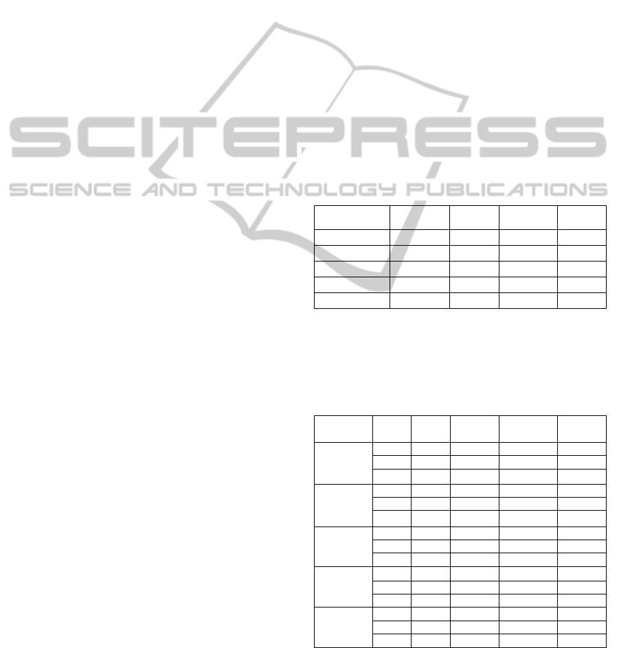
Table 1: Results of GA performance evaluation.
Crossover
Average performance
1-point
[0.507, 0.915] / 0.760
2-point
[0.132, 0.821] / 0.479
UE
[0.645, 0.957] / 0.834
UT
[0.309, 0.919] / 0.612
UP
[0.269, 0.938] / 0.657
UR
[0.624, 0.974] / 0.839
Table 1 contains the reliability of the algorithms
averaged over the 14 test problems from (Finck,
Hansen, Ros, and Auger, 2009) each solved 1000
times, and over all settings of the other (except
crossover) operators (selection, mutation, etc.). The
reliability is the percentage of the algorithm’s runs
that give satisfactorily precise solutions. In Table 1,
row headers "1-point, 2-point, UE, UT, UP, UR"
indicate the type of crossover, respectively, 1-point,
2-point, uniform equiprobable, uniform tournament-
based, uniform fitness proportional and uniform
rank-based crossovers.
Numbers in brackets demonstrate the variance of
these indicators. The first number in brackets is the
minimal value among the 14 tests; the second
number in brackets is the maximal value among the
14 tests. The last number is the corresponding
indicator averaged over 14 test functions.
After multiple runs and statistical processing of
the results, the following observations were found
(in terms of algorithm reliability). The best variants
are the new rank-based and conventional
(equiprobable) uniform operators. Tournament-
based crossover seems to be weak but it is the only
operator having maximum reliability of 100% on
some test problems where other operators fail.
Table 2: Comparison results of SelfCGA and problem
single best algorithms.
No
Crossover
Average
Min
Max
1
UE
0.818
0.787
0.894
SelfCGA
0.886
2
UE
0.841
0.808
0.903
SelfCGA
0.866
3
UE
0.901
0.887
0.921
SelfCGA
0.901
4
UR
0.925
0.877
0.959
SelfCGA
0.976
5
UT
0.950
0.901
1.00
SelfCGA
1.000
6
UE
0.953
0.861
0.999
SelfCGA
1.00
7
UT
0.897
0.832
0.927
SelfCGA
0.878
8
UR
0.741
0.667
0.800
SelfCGA
0.830
9
UT
0.967
0.917
0.983
SelfCGA
0.987
10
UE
0.853
0.803
0.891
SelfCGA
0.884
11
UR
0.821
0.734
0.888
SelfCGA
0.892
12
UR
0.833
0.765
0.881
SelfCGA
0.897
13
UR
0.956
0.902
0.998
SelfCGA
1.000
14
UR
0.974
0.935
0.999
SelfCGA
1.000
The next stage in evaluating the algorithms is a
comparison with the proposed self-configuring GA
(SelfCGA). Below in Table 2 one can find the
ICINCO 2012 - 9th International Conference on Informatics in Control, Automation and Robotics
90
results comparing SelfCGA with the single best
algorithm having had the best performance on the
corresponding problem.
Saying "single" algorithm, we mean the group of
algorithms with the same crossover operator but
with all variants of other settings. The average
reliability of this "single" algorithm is averaged over
all possible settings. "Min" and "Max" mean GA
settings given the worst and the best performance on
the corresponding test problem.
Analyzing Table 3, we can see that in four cases
(1, 2, 3, 10, numbers are given in italics) SelfCGA
demonstrates better reliability than the average
reliability of the corresponding single best algorithm
but worse than the maximal one. In one case (7
th
problem), the single best algorithm (with
tournament-based uniform crossover) gives better
average performance than SelfCGA. In the
remaining 9 cases (numbers are given in bold)
SelfCGA outperforms even the maximal reliability
of the single best algorithm.
Having described these results, one can conclude
that the proposed way of GA self-configuration not
only eliminates the time consuming effort for
determining the best settings but also can give a
performance improvement even in comparison with
the best known settings of conventional GA. It
means that we may use the SelfCGA in real world
problems solving.
8 SELF-CONFIGURING
GENETIC ALGORITHM
APPLICATION IN
SPACECRAFT CONTROL
SYSTEM DESIGN
The described algorithm Self-CGA is a suitable tool
for the application in hard optimization problems
that arise in spacecraft control systems design.
First of all we evaluate its performance on the
simplified models of technological and command-
programming control contours with 5 states.
To choose an effective variant of the
technological control contour we have to optimize
the algorithmically given function with 6 discrete
variables. The optimization space contains about
1.67∙10
7
variants and can be enumerated with an
exhaustive search within a reasonable time. In such a
situation, we know the best (k
*
) and the worst (k
-
)
admissible values of indicators. Executing 100 runs
of the algorithm, we will also know the worst value
of indicators (k
*
) obtained as a run result. The best
result of the run should be (k
*
) if the algorithm finds
it. We use 20 individuals in one generation and 30
generations for one run. This means the algorithm
will examine 600 points of the optimization space,
i.e. about 0.0036% of it. As the indicators of the
algorithm performance we will use the reliability
(the percentage of the algorithm’s runs that give the
exact solution k
*
); maximum deviation MD (the ratio
of k
*
- k
*
and k
*
in percentage to the last); and relative
maximum deviation RMD (the ratio of k
*
- k
*
and k
*
-
k
-
in percentage to the last). The comparison is made
for 5 algorithms, namely 4 conventional GAs with
new uniform crossover operators (UE, UR, UP, UT)
and SelfCGA. For conventional GAs, the results are
given for the best determination of all other settings.
In Table 3 below, the results are shown together
with the estimation of the computational efforts (the
number of generations needed to find the exact
solution averaged over successful runs, “Gener.”).
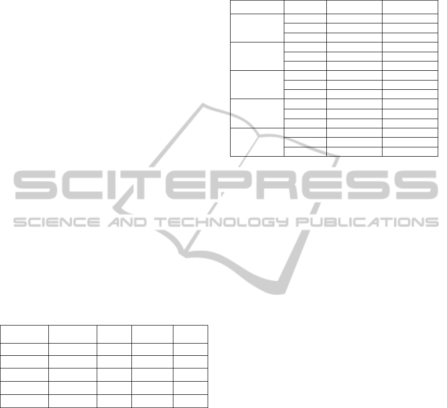
Table 3: Algorithm reliability comparison for
technological control contour model with 5 states
(spacecraft readiness coefficient).
Algorithm
Reliability
MD (%)
RMD (%)
Gener.
UE
0.89
0.0021
0.3576
26
UR
0.92
0.0017
0.2895
22
UP
0.84
0.0024
0.4087
26
UT
0.97
0.0009
0.1533
23
SelfCGA
0.98
0.0003
0.051
21
Similar evaluations for all 3 indicators of the
command-programming contour are given in Table
4 below.
Table 4: Algorithm reliability comparison for command-
programming control contour model with 5 states.
Algorithm
Ind.
Rel.
MD (%)
RMD (%)
Gener.
UE
T
0.87
6.431
9.028
26
t
1
0.76
0.956
3.528
43
t
2
0.83
13.392
26.01
28
UR
T
0.95
3.987
5.6
21
t
1
0.93
0.341
1.258
39
t
2
0.93
11.347
22.04
26
UP
T
0.79
6.667
9.359
28
t
1
0.71
1.156
4.266
45
t
2
0.74
16.321
31.7
29
UT
T
0.91
4.873
6.84
23
t
1
0.81
0.956
3.528
44
t
2
0.86
13.392
26.01
25
SelfCGA
T
0.99
3.245
4.555
19
t
1
0.96
0.1226
0.4524
33
t
2
0.98
9.987
19.397
17
The difference exists in the optimization
problem size. 600 evaluations of the objective
function correspond to 0.057% of the whole
Spacecrafts' Control Systems Effective Variants Choice with Self-configuring Genetic Algorithm
91
optimization space as the model has only 5 discrete
variables (about 10
6
variants).
From Table 3 and Table 4 one can see that Self-
CGA outperforms the alternative algorithms for all
problem statements and with all performance
measures.
Now we have to evaluate the performance of the
suggested algorithm on generalized models which
have much higher dimensions.
The optimization model for the technological
control contour has 11 discrete variables. The
corresponding optimization space contains about
1.76∙10
13
points and cannot be enumerated with an
exhaustive search especially if one recalls that the
examination of one point includes solving a linear
equations system with 40 variables. The best (k
*
)
and the worst (k
-
) admissible values of indicators
cannot be given and we use here their best known
evaluations after multiple runs consuming much
computational resources. Nevertheless, we still can
try to obtain the resulting table similar to Table 3
with statistical confidence. For the algorithms
performance evaluations we use 40 individuals for
one generation and 80 generation for one run that
examines about 1.82∙10
-7
% of the search space
examination. Results of numerical experiments are
summarized in Table 5.
Table 5: Algorithm reliability comparison for
technological control contour model with 40 states
(spacecraft readiness coefficient).
Algorithm
Reliability
MD (%)
RMD (%)
Gener.
UE
0.79
0.0115
0.2178
56
UR
0.86
0.0099
0.1875
48
UP
0.73
0.0121
0.2292
59
UT
0.87
0.0095
0.1799
49
SelfCGA
0.90
0.0092
0.1742
33
For the last problem, i.e. for the model of the
command-programming control contour with 96
states and more than 300 transitions, we cannot give
detailed information as we did above. This problem
has 13 variables and contains 4.5∙10
15
points in the
optimization space. It requires enormous
computational efforts to find reliable evaluations of
the necessary indicators. Instead, we give a smaller
table without MD and RMD measures. It gives us
some insight on the comparative reliability of the
investigated algorithms. The algorithms performance
evaluation requires the examination of 2.2∙10
-10
% of
the search space (100 individuals and 100
generations). Results averaged over 20 runs are
summarized in Table 6.
Table 6: Algorithm reliability comparison for command-
programming control contour model with 96 states.
Algorithm
Indicator
Reliability
Generation
UE
T
0.76
65
t
1
0.67
81
t
2
0.75
69
UR
T
0.84
59
t
1
0.81
78
t
2
0.84
64
UP
T
0.70
69
t
1
0.59
76
t
2
0.63
72
UT
T
0.83
61
t
1
0.72
85
t
2
0.77
66
SelfCGA
T
0.91
58
t
1
0.87
75
t
2
0.89
53
Table 5 and Table 6 show that the Self-CGA
outperforms all alternative algorithms.
When solving these problems for real we only
need one run, but that one run requires much more
computation power than any single run above.
9 CONCLUSIONS
In this paper, the mathematical models in the form
of Markov chains have been developed and
implemented for choosing effective variants of
spacecraft control contours. These models contain
tens of states and hundreds of transitions that make
the corresponding optimization problems hard to
solve.
It is suggested to use the genetic algorithms in
such a situation because of their reliability and high
potential to be problem adaptable. As GAs
performance is highly dependent on their setting
determination and parameter tuning, the special self-
configuring GA is suggested that eliminates this
problem. The high performance of the suggested
algorithm is demonstrated through experiments with
test problems and then is validated by the solving
hard optimization problems. The self-configuring
genetic algorithm is suggested to be used for
choosing effective variants of spacecraft control
systems as it is very reliable and requires no expert
knowledge in evolutionary optimization from end
users (aerospace engineers). We did not try to
implement the best known GA with optimal
configuration and optimally tuned parameters.
Certainly, one could easily imagine that the much
better GA exists. However, it is a problem to find it
for every problem in hand. The way of the self-
configuration proposed in this paper that involves all
ICINCO 2012 - 9th International Conference on Informatics in Control, Automation and Robotics
92

variants of all operators can be easily expanded by
adding new operators or operator variants. The self-
configuring process monitoring gives the additional
information for further SelfCGA improving. E.g., if
the high level mutation is always the winner among
mutation variants then we can add some higher level
mutation operators in the competitors list instead of
lower level variants. Another example is the
possibility of 1-point and 2-point crossovers
removing from the crossover operators list that was
evident in our experiments.
The future research includes also not only
direct expansion in using the simulation models and
multicriterial optimization problem statements but
also the improvement of Self-CGA adaptability
through the population size control and adoption of
additional operators and operator variants.
ACKNOWLEDGEMENTS
The research is supported through the Governmental
contracts № 16.740.11.0742 and № 11.519.11.4002.
The authors are deeply grateful to Dr. Linda Ott,
a professor at the Technological University of
Michigan, for her invaluable help in improving the
text of the article.
REFERENCES
Angeline, P. J., 1995. Adaptive and self-adaptive evolutionary
computations. In: Palaniswami M. and Attikiouzel Y.,
editors, Computational Intelligence: A Dynamic Systems
Perspective, pp. 152–163. IEEE Press.
De Jong, K. A., Spears, W., 1991. On the Virtues of
Parameterized Uniform Crossover. In: Richard K.
Belew, Lashon B. Booker, editors, Proceedings of the
4th International Conference on Genetic Algorithms,
pp. 230-236. Morgan Kaufmann.
Eiben, A. E., Smith, J. E., 2003. Introduction to
evolutionary computing. Springer-Verlag, Berlin,
Heidelberg.
Eiben, A. E., Hinterding, R., and Michalewicz, Z., 1999.
Parameter control in evolutionary algorithms. In: IEEE
Transactions on evolutionary computation, 3(2):124-141.
Finck, S., Hansen, N., Ros, R., and Auger, A., 2009. Real-
parameter black-box optimization benchmarking
2009: Presentation of the noiseless functions.
Technical Report 2009/20, Research Center PPE.
Gomez, J., 2004. Self-Adaptation of Operator Rates in
Evolutionary Algorithms. In Deb, K. et al., editors,
GECCO 2004, LNCS 3102, pp. 1162–1173.
Haupt, R. L., Haupt, S. E., 2004. Practical genetic
algorithms. John Wiley & Sons, Inc., Hoboken, New
Jersey.
Meyer-Nieberg, S., Beyer, H.-G., 2007. Self-Adaptation in
Evolutionary Algorithms. In: F. Lobo, C. Lima, and Z.
Michalewicz, editors, Parameter Setting in
Evolutionary Algorithm, pp. 47-75.
Semenkin, E. S., Semenkina, M. E., 2007. Application of
genetic algorithm with modified uniform
recombination operator for automated implementation
of intellectual information technologies. In: Vestnik.
Scientific Journal of the Siberian State Aerospace
University named after academician M. F. Reshetnev.
– 2007. – Issue 3 (16). – Pp. 27-32. (In Russian,
abstract in English).
Syswerda, G., 1989. Uniform crossover in genetic
algorithms, In: J. Schaffer, editor, Proceedings of the
3
rd
International Conference on Genetic Algorithms,
pp. 2-9. Morgan Kaufmann.
Spacecrafts' Control Systems Effective Variants Choice with Self-configuring Genetic Algorithm
93
