Low-speed Modeling and Simulation of Torpedo-shaped AUVs
Bjarni Helgason
1
, Leifur Leifsson
1
, Indridi Rikhardsson
1
, Helgi Thorgilsson
2
and Slawomir Koziel
3
1
CADIA/Laboratory for Unmanned Vehicles, School of Science and Engineering, Reykjavik University, Reykjavik, Iceland
2
Teledyne Gavia ehf, Vesturvor 29, 200 Kopavogur, Iceland
3
Engineering Optimization & Modeling Center, School of Science and Eng., Reykjavik University, Reykjavik, Iceland
Keywords:
Autonomous Underwater Vehicle, Low-speed Motion, Vehicle Dynamics, Simulation, Experimental Valida-
tion.
Abstract:
Autonomous underwater vehicles (AUVs) have become important in many marine engineering applications,
such as environmental monitoring, pipeline inspections, or oceanography. For these types of applications, most
of the AUVs available in both academia and industry are shaped like a torpedo and travel at speeds of 3 knots
or higher. There is an growing interest in AUVs that are capable of performing tasks at both low-speed as well
as high speeds. Currently, many torpedo-shaped AUVs are not capable of controlled low-speed motion. This
paper presents a simulation model for the low-speed motion of torpedo-shaped AUVs. The model is capable
of simulating the surge, sway, heave, and yaw motions. The hydrodynamic forces acting on the AUV hull are
modelled using strip theory, experimental data, and computational fluid dynamics. The simulation model was
implemented using a commercially available software and validated using experimental data obtained from
the Gavia AUV. The results show that the simulation model captures the AUV motion at low-speed and agrees
well with the experimental data.
1 INTRODUCTION
An autonomous underwater vehicle (AUV) is a robot
which travels underwater without requiring any input
from an operator (Fossen, 1994). The tasks and mis-
sions of AUVs are constantly evolving and becom-
ing increasingly important for commercial-, military-,
research- and hobby users. A typical commercial job
for an AUV is, e.g., to construct detailed maps of the
seafloor before building subsea infrastructure in the
oil and gas industry. A typical military mission for an
AUV is to map an area and determine if there are any
mines, or to monitor a protected area for unidentified
objects. Scientists use AUVs to study lakes, the ocean
and the ocean floor.
Numerous AUVs have been developed, both in
academia, e.g., (Clark et al., 2009; Ananthakrishnan
and Decron, 2000; de Barros et al., 2008; Kennedy,
2002), and in the industry, e.g., (Allen et al., 2000).
These vehicles are of various shapes and sizes. AUV’s
intended for high-speed (higher than 3 knots) and
long-range (longer than 6 hours) missions are com-
monly torpedo-shaped with aft-mounted propulsion
and control systems (Braunl et al., 2007; Eastman
et al., 2009). AUVs designed for performing tasks at
low speeds differ, but (usually) their shapes are not
streamlined, as it is not necessary. However, they
are (normally) equipped with several thrusters for ma-
noeuvring in all directions. There is an growing inter-
est in AUVs that are capable to perform tasks at both
low- (or zero) and high-speeds (Braunl et al., 2007).
Currently, many torpedo-shaped AUVs are not capa-
ble of controlled low-speed motion.
The objective of this research is to investigate the
low-speed characteristics of torpedo shaped AUVs
and their control. In particular, we model the ve-
hicle motion at low-speed and develop a computa-
tional framework capable of simulating the vehicle
response. We use the commercially available Gavia
AUV
1
as a testbed (Fig. 1). The model is validated
and tuned using data from physical experiments.
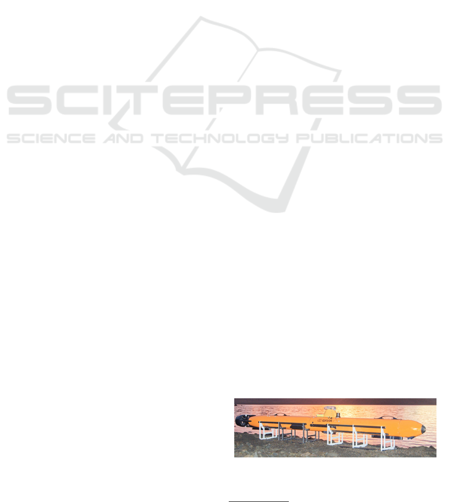
Figure 1: The Gavia AUV is commercially available and
is capable of various missions, such as oceanography and
pipeline inspection.
1
www.gavia.is
333
Helgason B., Leifsson L., Rikhardsson I., Thorgilsson H. and Koziel S..
Low-speed Modeling and Simulation of Torpedo-shaped AUVs.
DOI: 10.5220/0004047103330338
In Proceedings of the 9th International Conference on Informatics in Control, Automation and Robotics (ICINCO-2012), pages 333-338
ISBN: 978-989-8565-22-8
Copyright
c
2012 SCITEPRESS (Science and Technology Publications, Lda.)
2 GOVERNING EQUATIONS FOR
LOW-SPEED MOTION
We want to move the AUV in certain directions dur-
ing low-speed motion. In particular, we want to move
the AUV back and forth, up and down, to the sides,
and rotate it. Therefore, only four degrees of freedom
are required. In this section, we describe the govern-
ing equations for such motion and we develop specific
models for the system dynamics.
2.1 General Equations and Frames of
Reference
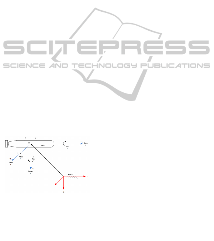
Two coordinate frames must be defined to describe
the motion of underwater vehicles (Fig. 2). The mov-
ing coordinate frame X
0
Y
0
Z
0
is fixed to the vehicle
and is called the body-fixed reference frame and the
fixed coordinate frame XY Z is the earth coordinate
system (Fossen, 1994). The fixed coordinate system
is an earth coordinate system while the moving one
follows vehicle heading and location each time. The
X−axis is in line with length of vehicle and center of
gravity, where positive movement means forward and
vice versa. All movement in line with the X −axis
is surge (u is surge velocity) movement, while rota-
tion about the axis is roll (p) rotation. Axes Y and Z
then follow the X−axis as in a regular coordinate sys-
tem. Movement in line with Y -axis is sway (v is sway
velocity), while rotation about same axis is pitch (q)
rotation. Movement in line with Z-axis is heave (w is
heave velocity), while rotating about same axis is yaw
(r) rotation.
Figure 2: Coordinate systems, both body-fixed and earth-
fixed.
At low speed, the AUV moves in one direction at
a time. In particular, the AUV moves along the axes
of surge, sway and heave, and rotates (yaws) about
heave axis. The general governing equations of mo-
tion along each of these axes are (Fossen, 1994)
m
˙u − vr + wq −x
G
(q
2
+ r
2
) + y
G
(pq − ˙r)
+z
G
(pr + ˙q)] =
∑
X
ext
(1)
m
˙v − wp + ur − y
G
(r
2
+ p
2
) + z
G
(qr − ˙p)
+x
G
(qp + ˙r)] =
∑
Y
ext
(2)
m
˙w − uq +vp − z
G
(p
2
+ q
2
) + x
G
(rp − ˙q)
+y
G
(rq + ˙p)] =
∑
Z
ext
(3)
I
z
˙r +(I
y
− I
x
)pq + m [x
g
( ˙v − wp + ur) − y
G
( ˙u − vr + wg)] =
∑
N
ext
(4)
where m is the rigid body mass, I is the rigid body
inertia about a specific axis, x
G
, y
G
and z
G
are each
axis distance from the rigid body center of gravity,
X
ext
, Y
ext
, Z
ext
are forces acting of the vehicle in their
respective axes, and N
ext
is the moment about the
Z
0
−axis.
We will now analyze each of these equations for
the low-speed motion of torpedo-shaped AUVs.
2.2 Surge Motion
The external forces acting on the AUV in the surge
direction are due to the thrust, drag and added mass.
The governing surge equation of motion, Eq. (1),
becomes, when taking into account these external
forces, as well as neglecting motion in other direc-
tions,
m ˙u = −X
˙u
˙u − D
surge
u + T
surge
, (5)
where X
˙u
is the added mass derivative for surge, D
surge
is the hydrodynamic drag for surge, and T
surge
is the
surge thrust force. Effects due to Coriolis and cen-
tripetal forces are neglected.
In this work, we estimate the added mass deriva-
tives using strip theory for slender bodies (Fossen,
1994). The added mass derivative for surge is (Hel-
gason, 2012)
X
˙u
' −0.1m. (6)
The hydrodynamic drag is modelled as (Wang and
Clark, 2007)
D = D
L
+ D
Q
, (7)
where D
L
and D
Q
are the linear and quadratic drag
terms, respectively. The linear term is determined by
experiments, and the quadratic term is
D
Q
= C
D
surge
1
2
ρA
surge
u|u|, (8)
ICINCO2012-9thInternationalConferenceonInformaticsinControl,AutomationandRobotics
334

where C
D
surge
is the drag coefficient for surge motion,
ρ is the water density, A
surge
is the reference area for
surge motion. The surge drag coefficient is deter-
mined using computational fluid dynamics (CFD) and
the resulting value is C
D
surge
= 0.37 (Helgason, 2012).
2.3 Sway Motion
Same type of forces act on the AUV in the sway direc-
tion as in the surge one. The governing sway equation
of motion, Eq. (2), becomes (Helgason, 2012)
m ˙v = −Y
˙v
˙v − D
sway
v + T
sway
, (9)
where Y
˙v
is the added mass derivative for sway, D
sway
is the hydrodynamic drag for sway, and T
sway
is the
sway thrust force. Strip theory yields the added mass
derivative as (Helgason, 2012)
Y
˙v
' −πρR
2
L, (10)
where R is the maximum radius of the AUV hull and L
is it’s length. The drag is modelled in the same way as
for the surge motion, i.e., Eqs. (7) and (8). However,
the quadratic drag coefficient in the sway direction
is estimated based on experimental data for circular
cylinder in cross-flow and is taken to be C
D
sway
= 1.2
(White, 2008).
2.4 Heave Motion
In the heave direction, the same external forces act
on the vehicle as in the surge and sway directions,
including the gravitational and buoyancy forces. The
governing heave equation of motion, Eq. (3), is then
(Helgason, 2012)
m ˙w = −Z
˙w
˙w − D
heave
w − ( f
g
+ f
b
) + T
heave
, (11)
where Z
˙w
is the added mass derivative for heave,
D
heave
is the hydrodynamic drag for heave, f
g
is the
vehicle weight, f
b
is the vehicle buoyancy force, and
T
heave
is the heave thrust force. The added mass
derivative term Z
˙w
for heave can be assumed to be
the same as for sway, Eq. (10), because of symmetry
in the torpedo-shaped hull. For the same reason, we
use the same drag coefficient value, i.e., C
D
heave
= 1.2.
2.5 Yaw Motion
External moments in the yaw rotational motion are
moments due to the thrusters, hull drag, and added
mass. The governing equation for yaw motion, Eq.
(2), becomes (Helgason, 2012)
I
z
˙r = −D
yaw
r +M
yaw
, (12)
Heave ModelSurge Model Sway Model
Yaw Model
Figure 3: The four non interacting models of the simulator
for each of the degrees of freedom.
where D
yaw
is the hydrodynamic drag for yaw, and
M
yaw
is the yawing moment due to the thrusters. The
drag is modelled using Eqs. (7) and (8). The quadratic
drag coefficient is estimated based on experimental
results for cylinder in cross-flow. We assume that
each half of the cylinder is in cross-flow with the re-
sulting force acting in it’s center. Based on this the
drag coefficient is found to by C
D
yaw
= 0.55 (White,
2008).
3 SIMULATOR FRAMEWORK
The simulator was built in a plain block diagram en-
vironment using Simulink (Mathworks, 2011) where
the differential equations for each degree of freedom
(DOF) presented in Section 2 were implemented. The
simulator structure is based on four non interacting
models, each corresponding to a separate DOF (Fig.
3). Motion of the AUV along each DOF is simulated
at a time and the combination of all the four models
yields a simulation of the overall motion.
Due to length limitations, the models cannot be
described in detail. However, the general structure of
each model is shown in Fig. 4. The first block on
the left is the input signal generator. In the second
block, the thruster characteristics are defined. The
main thruster at the rear is used for surge motion,
while different thrusters are used for the other DOF’s.
Input Thrusters
External
Forces
AUV
Dynamics
Output
Feedback
+
-
Figure 4: The basic block structure for each of the simula-
tion models.
The third block represents the external forces acting
on the AUV, such as drag, added mass, gravity, and
buoyancy. The fourth block represents the AUV dy-
namics, which is different for each DOF, as described
in Section 2. The block farthest to the right pro-
duces the simulation output, such as depth, heading
Low-speedModelingandSimulationofTorpedo-shapedAUVs
335
and position. The bottom block represents the feed-
back from the sensors (including any time delays). A
detailed description of each model is given in (Helga-
son, 2012).
4 EXPERIMENTAL TESTING
In order to gather data for validating and tuning the
simulator, several experiments were performed using
the Gavia AUV. In this section, we describe the exper-
imental approach and setup for open and closed loop
testing.
4.1 Approach
The simulator can handle AUV motion in surge, sway,
heave, and yaw. Therefore, data on the vehicle be-
haviour in all those directions is required for the sim-
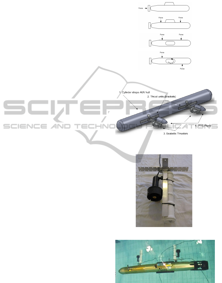
ulator validation. Figure 5 shows where forces are
needed for each direction. The testbed AUV only
has a rear mounted propeller and can, therefore, only
move in the surge direction. Additional thrusters were
mounted on to the hull to achieve the desired motion.
For each direction, both the open and closed loop per-
formance were studied. In particular, we studied the
response as a function of the thruster load, as well as
different PID controller settings.
4.2 Setup
A pair of externally mounted thrusters were used
for the experimental testing, aside the case of surge,
where the rear mounted propeller was used. The
thrusters were installed on a bracket which was
mounted on the sides of the AUV hull as shown in Fig.
6. A plastic pipe was included in the bracket to pro-
vide buoyancy to balance the weight of the thruster.
The thrusters are manufactured by Seabotix and are
controlled by a Devantech MD22 motor controller.
Figure 7 shows a thruster mounted on the bracket.
Figure 8 shows the Gavia AUV with two thrusters
mounted on it’s side for sway testing. All tests were
performed in an indoor swimming pool of 3 m depth.
5 MODEL VALIDATION AND
TUNING
In this section, we present the results obtained in the
experiments described in Section 4 and compare them
with numerical results obtained by the model pre-
sented in Sections 2 and 3. In particular, we present
Surge
Sway
Heave
Yaw
Figure 5: Experimental setup of the forces acting on the
AUV hull for testing of each of the degree of freedom.
Figure 6: A sketch of the bracket and thrusters mounted on
the hull of the AUV.
Figure 7: An assembly of the thruster, bracket and float.
Figure 8: The Gavia AUV with the thruster assembly
mounted on the sides during testing.
results for surge, sway, and yaw motions. The heave
model is identical to the sway model.
ICINCO2012-9thInternationalConferenceonInformaticsinControl,AutomationandRobotics
336
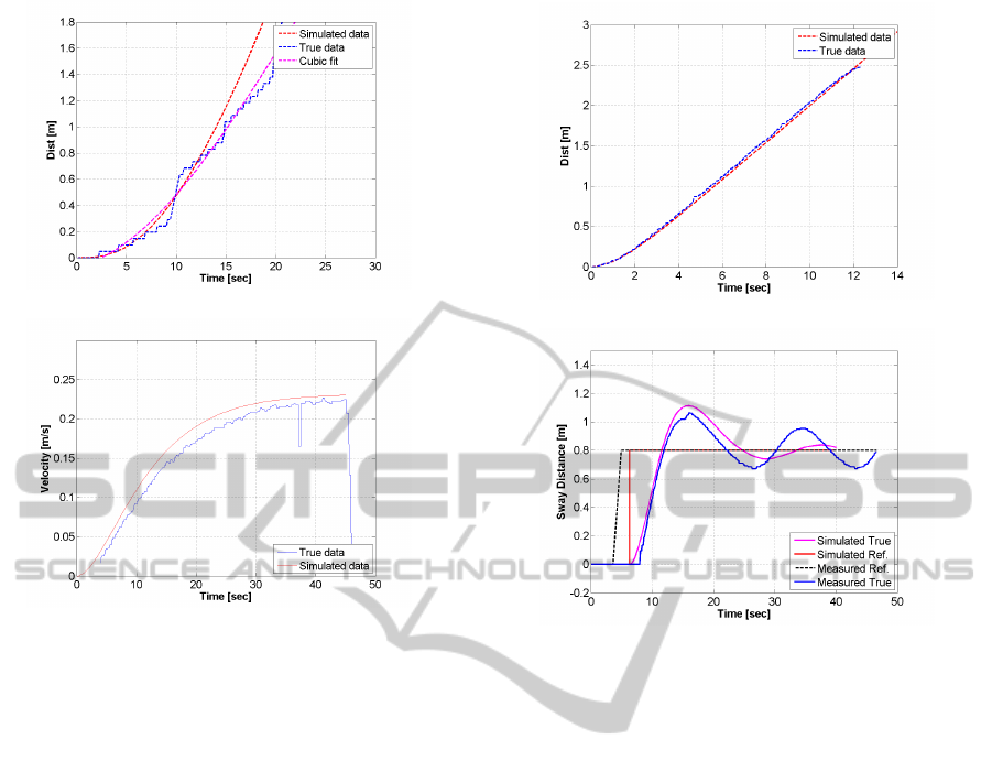
(a)
(b)
Figure 9: Surge open loop response for the propeller at 197
rpm (a) distance as a function of time, here the cubic fit is a
polynomial fit to the true data used for comparison with the
simulation, and (b) velocity as a function of time.
5.1 Surge
Open loop response for surge forward motion are
shown in Fig. 9 for the propeller at 197 rpm. A multi-
plicative tuning factor was applied to the model. The
simulation model follows the experimental data for
the first 12 seconds or so. The discontinuous shape of
the experimental data is due to a low sampling rate of
the sensors.
5.2 Sway
Open and closed loop sway responses are shown in
Fig. 10. Here the quadratic drag term was tuned with
a multiplicative constant to match the data in the open
loop response. In the closed loop test, the AUV was
translated by 80 cm.
The results show that the control system is able to
quickly reach the translated distance, but overshoots
by approximately 23 cm and converges towards the
reference value slowly. The simulator follows the ex-
perimental results quite well, but overshoots by 30
cm, and converges more quickly towards the refer-
ence value. This indicates the discrepancy between
the experimental and simulation configurations.
(a)
(b)
Figure 10: Sway responses (a) open loop with constant
thrust of 0.5, and (b) closed loop with PID values of P = 30,
I = 0, and D = 0.
5.3 Yaw
Open and closed loop yaw responses are shown in
Fig. 11. Here, as in the case of sway, the quadratic
drag term was tuned with a multiplicative constant
to match the data in the open loop response. In the
closed loop test, the AUV was rotated by 40 degrees.
The results show that the control system quickly
rotates the AUV towards the reference value, but over-
shoots by about 14 degrees. However, it recovers
swiftly and reaches the reference value within 15 to
20 seconds. The simulation follows the data closely
throughout the data series.
6 CONCLUSIONS
A simulation model for the motion of torpedo-shaped
AUVs at low-speed was presented. The model is
based the general equations of motion for marine ve-
hicles. The hydrodynamic forces acting on the AUV
hull were modelled using strip theory, experimental
data, and computational fluid dynamics. The simu-
lation model was implemented using a commercially
available software and validated using experimental
Low-speedModelingandSimulationofTorpedo-shapedAUVs
337
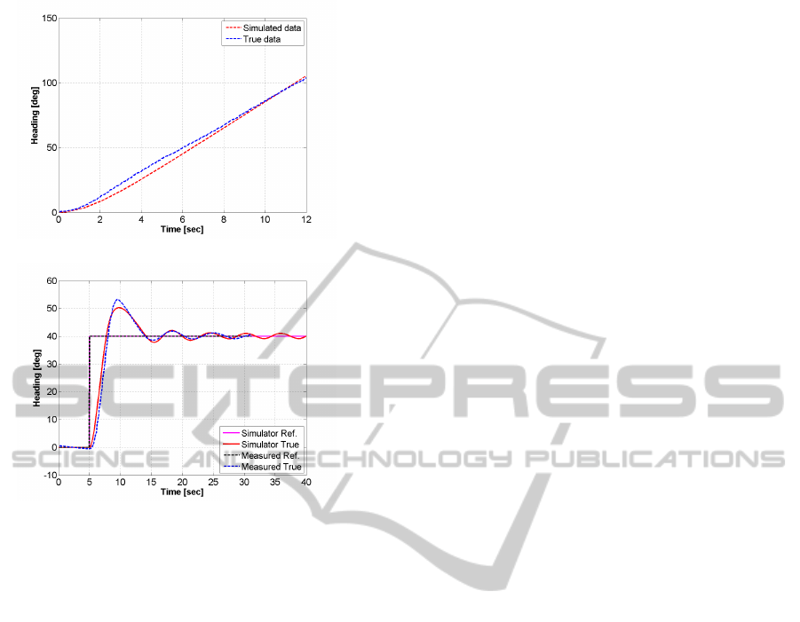
(a)
(b)
Figure 11: Yaw responses (a) open loop with constant thrust
of 0.5, (b) closed loop with PID values of P = 2, I = 0, and
D = 0.
data obtained from a commercially available AUV.
The results show that the simulation model captures
the AUV motion at low-speed and compares well with
the experimental data.
The results of the research are promising and sug-
gest that torpedo-shaped AUVs can be effectively
controlled at low-speed with only a few thrusters. The
next step in our work is to construct modules for the
testbed AUV which contain thrusters within them. In-
corporate these modules into the AUV and repeat the
experimental testing. In the future, we will consider
what type of thrusters are most suitable, i.e., the typi-
cal propeller thrusters, or more novel devices, such as
vortex ring generators or pulsating membranes.
ACKNOWLEDGEMENTS
We would like to thank the University of Iceland for
lending us their Gavia AUV to perform the experi-
ments. We would also like to acknowledge the staff
at Teledyne Gavia ehf. for their assistance during this
work.
REFERENCES
Allen, B., Vorus, W., and Prestero, T. (2000). Propulsion
system performance enhancements on remus auvs. In
OCEANS 2000 MTS/IEEE Conference and Exhibi-
tion, volume 3, pages 1869–1873. IEEE.
Ananthakrishnan, P. and Decron, S. (2000). Dynamic sta-
bility of small and mini-autonomous underwater vehi-
cles: Part i. analysis and simulation for mid water ap-
plications. Technical report, Technical Report, Florida
Atlantic University, Florida.
Braunl, T., Boeing, A., Gonzalez, L., Koestler, A., and
Nguyen, M. (2007). Design, modelling and simulation
of an autonomous underwater vehicle. International
Journal of Vehicle Autonomous Systems, 4, 2(3):106–
121.
Clark, T., Klein, P., Lake, G., Lawrence-Simon, S., Moore,
J., Rhea-Carver, B., Sotola, M., Wilson, S., Wolf-
skill, C., and Wu, A. (2009). Kraken: Kinematically
roving autonomously kontrolled electro-nautic. 47th
AIAA Aerospace Sciences Meeting Including the New
Horizons Forum and Aerospace Exposition, Orlando,
Florida.
de Barros, E., Dantas, J., Pascoal, A., and de S
´
a, E.
(2008). Investigation of normal force and moment co-
efficients for an auv at nonlinear angle of attack and
sideslip range. IEEE Journal of Oceanic Engineering,
33(4):538–549.
Eastman, D., Lambrechts, P., and Turevskiy, A. (2009). De-
sign and verification of motion control algorithms us-
ing simulation. Embedded Systems Conference, pages
1–4.
Fossen, T. (1994). Guidance and Control of Ocean Vehicles.
John Wiley & Sons.
Helgason, B. (2012). Low speed modeling and simulation
of gavia auv. Master’s thesis, Reykjavik University.
Kennedy, J. (2002). Decoupled modelling and controller de-
sign for the hybrid autonomous underwater vehicles:
Maco. Master’s thesis, Univeristy of Victoria.
Mathworks (2011). Simulink/Matlab.
Wang, W. and Clark, C. (2007). Modeling and simulation
of the Videoray Pro III underwater vehicle. OCEANS
2006-Asia Pacific, pages 1–7.
White, F. M. (2008). Fluid Mechanics. McGraw-Hill, 6
edition.
ICINCO2012-9thInternationalConferenceonInformaticsinControl,AutomationandRobotics
338
