
Comparing Adaptive and Non-adaptive Models of Cargo
Transportation in Multi-agent System for Real Time Truck
Scheduling
Oleg Granichin
1
, Petr Skobelev
2
, Alexander Lada
2
, Igor Mayorov
2
and Alexander Tsarev
2
1
Saint Petersburg State University, Saint Petersburg, Russia
2
Software Engineering Company «Smart Solutions», Ltd., Samara, Russia
Keywords: Multi-agent Systems, Adaptive Scheduling, Trucks, Cargo Transportation, Simulation, Real-time, Mobile
Resources.
Abstract: The application of multi-agent platform for real-time adaptive scheduling of trucks is considered. In case of
unpredictable events the system works adaptively and doesn’t stop to restart the plan from the beginning.
Different models of cargo transportation for truck companies having own fleet are analysed. The results
show that using adaptive scheduling in real time it is possible to create significantly more profitable
schedules (up to 40-60% compared with rigid models) and save a number of trucks (up to 20%) for the same
amount of orders.
1 INTRODUCTION
The problem of resource optimize allocation are
usually solved, when all the orders and resources are
given in advance and don’t change in the process of
scheduling. In these cases classical batch planning
methods can be used characterized by the time-
consuming full combinatorial search or different
types of heuristics requiring a lot of computational
power (Leung, 2004); (Bonabeau, 2000).
Any change is considered as a need for full
change of schedule, which have to be processed
from scratch. But for solving real-life problems of
resource allocation, existing approaches do not work
at all or produce unfeasible schedules which require
exhausting manual re-work for dispatchers.
For solving such problems we apply multi-agent
technology (Wooldridge, 2002). The approach we
are working on is based on Demand-and-Resource
Networks (DRN) of agents representing orders and
resources (Skobelev, 2011). That allows us to find a
‘well-balanced’ solution acceptable for all the agents
as well as for company as a whole.
As a result of such interactions of agents a near-
to-optimal (acceptable) solution of the problem is
achieved in the form of ‘not-stable equilibrium’,
which can be adaptively corrected in real time after
each new incoming event representing new order or
order cancellation, truck breakdown, delay of work
execution, etc. The developed multi-agent
technology allows us to solve complex resource
allocation, when the number of orders and resources
is not given in advance and there is a high dynamics
of occurring events (Ivashenko, 2011).
The results of the research are important for the
future developments of intelligent freight
management systems and dispatching of any other
mobile resources that are able to operate in real time.
2 THE MODELS OF
TRANSPORTATION PROCESS
ORGANIZATION
Let’s assume that we have a fleet of M trucks based
in certain cities in a transportation network. The
operation cost of each truck is given. Orders come
into the system with the specified points of loading
and unloading, loading start time, unloading finish
time, price and penalties for delays when a loading
or unloading is done later than they should.
Distances between points are also given and
described by a matrix of distances.
The objective is to schedule the trucks in real
time and determine transportation company profit
282
Granichin O., Skobelev P., Lada A., Mayorov I. and Tsarev A..
Comparing Adaptive and Non-adaptive Models of Cargo Transportation in Multi-agent System for Real Time Truck Scheduling.
DOI: 10.5220/0004148602820285
In Proceedings of the 4th International Joint Conference on Computational Intelligence (ECTA-2012), pages 282-285
ISBN: 978-989-8565-33-4
Copyright
c
2012 SCITEPRESS (Science and Technology Publications, Lda.)

depending on the scheduling strategy (model) and
the number of trucks.
The optimization criterion of the task is the
maximal total profit of all the trucks in company
fleet. The research is done for four different models
of organization of transportation process including
not-adaptive and adaptive models described below.
The total profit of the fleet of trucks is calculated
as a sum of profits of each truck:
i
i
p
P .
(1)
The profit of one truck is:
,
'
j
ij
i
ij
i
j
i
t
q
t
q
c
p
t
(2)
where sum includes all orders j executed by the
truck i, c
j
– price of order j per time unit, q
i
– cost of
the truck per time unit, t
ij
– time of execution order j
by truck i, t’
ij
– empty run time for order j.
Let’s consider 4 models of transportation process
organization.
Model #1 – the ‘Returning to base after an order
execution’ model. After each order execution the
truck should return to the base point. Order is
assigned to a truck that has a ‘window’ in its
schedule during the order time period. If the loading
point of the order is a different city, then the truck
should arrive there at the loading time. No
reassignments of the trucks already assigned to the
orders are allowed.
Model #2 – the ‘No return to base after an order
execution’ model. After each order execution truck
stays at the order destination point, without returning
to base, and waits for a next order.
Model #3 – the ‘Delays with penalties’ model.
Orders can be scheduled with delays of time of
arrival at the loading point. In this case profit with
penalty calculation is:
,
'''
'
k
ik
k
ik
i
ik
k
k
j
ij
i
ij
i
j
i
t
p
t
q
t
q
c
t
q
t
q
c
p
t
(3)
where the sum by index j includes all orders that
were executed just in time by the truck i, the sum by
index k includes all orders that were executed with
delays t
’’
ik
, p
j
– penalty of each delay per time unit.
Model #4 – the ‘Adaptive scheduling with penalties’
model. It is equal to the previous model, but it
allows the truck reassignment when a profit from a
new order is higher than a profit from the previous
one.
3 THE MULTI-AGENT
SIMULATOR
A special multi-agent simulator (MAS) has been
created for modelling of adaptive real time
scheduling. It works as follows. Every truck is
associated with a truck agent, every order – with an
order agent. The agents are able to send and receive
messages and take decisions according to their logic
and current situation. The unified spatio-temporal
scale is defined to achieve visibility of results and
unified logic: time is counted from the moment of
the first order entry. The upper border of planning is
determined by the planning horizon, calculated in
days. The distances are brought to time scale by
division of the distances by the average speed.
When a new order comes, a request for its
allocation is sent to all the truck agents. ‘Candidates’
for re-scheduling (in case of increasing profit) are
ordered of the prospective profit. Then the order
agent chooses the truck that gives the maximal
profit. The profit is calculated as a difference
between the order revenue (price) and the order full
cost. When order implies an empty run to loading
point, its cost is also deducted from the revenue. In
case of strategy (model), where penalties are
applied, their influence on profit is analyzed. For
penalty is proportional to time of delay, the orders
with big delays will not be scheduled.
Let’s consider world of simulations for one
truck. There are 4 cities (points) given, among which
the distances are determined by the matrix (see
Table 1) in days of trip. Time of trip doesn’t
necessarily correspond to the distance, because of
roads quality.
At the beginning of the trip the truck is located in
the point 1. At different times cargo transportation
orders #1-5 to different points come into the system.
Duration of execution of an order is 1-2 days.
Scheduling horizon equals t = 10 days. The costs of
orders are calculated equally using company tariff as
c = 3 standard units (SU) / day, i.e. 2-days trip would
have cost of 6 SU. Idle time of a truck leads to daily
loss of q=0.3 SU.
Table 1: Matrix of distances among cities.
Point 1 Point 2 Point 3 Point 4
Point 1
0 1 1 2
Point 2
1 0 2 1
Point 3
1 2 0 1
Point 4
2 1 1 0
Daily running cost in case of empty run of truck
or order execution is q=1. Drivers are allowed to
ComparingAdaptiveandNon-adaptiveModelsofCargoTransportationinMulti-agentSystemforRealTimeTruck
Scheduling
283
execute orders with delays, but every day of delay
costs pp = 0.6 SU. Some orders are shifted to the
right on the time axis because of this. The aim is to
be able to schedule trips, as orders come in (the
orders are not known in advance) and calculate
profit. Orders are marked with a number according
to the place in the sequence of entry into the system
and characterized by time of their entry (moment of
entry t), moments of start and finish of order
execution, duration (in days), point of loading and
point of unloading (Table 2).
Table2: Parameters of orders.
Characteristics
Order number
1 2 3 4 5
Time of entry
1 3 5 6 7
Start time of execution
3 4 7 8 9
Finish time of execution
5 5 9 9 10
Where from
4 3 1 4 3
Where to
1 1 4 3 1
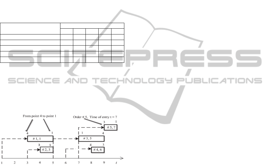
Figure 1 shows orders as rectangles, with the
order number and the time of entry. Above each
rectangle ‘where from – where to’ locations are
described. The start and the finish of each rectangle
correspond to the start and the finish of the order
execution.
Figure 1: Diagram of orders entry and scheduling.
Let’s calculate the profit of truck #1 in the Model
#3, where penalties are applied. We will calculate
the profit P at the moments of transition of the truck
from one state to another step by step.
Step 1. Execution of order #1 will require to start at
the moment t=1 from point #1 to point # 4 and will
take 2 days till the moment t=3. At the moment t=3
the profit is P=-q*2=-2.
Step 2. The transportation of cargo from point 4 to
the point 1 will take 2 days, and at t=5 the truck will
arrive at the point 1 with the profit P=-2+(c-q)*2=-
2+2*2=2. Assume that the truck agent assesses
options of further schedule and execution upon
arrival to point 1 at time t=5. Its profit at point 4 is
P=2. By this time order # 3 has been entered at the
moment of time #3. There are two options to execute
it:
Order #2 is to be executed with delay;
Order #2 is rejected, idle time cost is accepted,
order #3 from the same point 1 is to be taken; for
order # 2 can be executed with delay before
execution of order #3, no further options will be
taken into consideration. Let’s take a more precise
look at 2 options.
Step 3. Truck needs to reach point 3, moving from
point 1 (1 day trip), pick up the order and execute it,
going from point 3 to point 1 (1 day). The increase
of profit is dp=-1*q+(c-q)*1=-1+2=1.
Penalty applied because of delay is -pp*2=-2*0.6=-
1.2. As a result the truck will be at the moment t=7
at the point 1 with the profit P=2+1-1.2=1.8.
Execution of the order would seem to be
unprofitable, but one should take into consideration
that in case of cancellation of the order the truck
would stay idle for 2 days, and the profit at the
moment t=7 would be P=2-2*0.3=1.4.
Step 4. That’s why the truck agent is interested in
the execution of order #2 with delay, order #3, t=
7…9 (from point 1 to point 4) - 2 days, profit is
P=1.8+2*(c-q)=1.8+2*2=5.8, and the truck moves to
point 4.
Step 5. At the moment t=9 new order# 5 comes in
at the point 3 with start time of execution t=9; empty
run to its loading point is 1 day, what puts the order
beyond the 10-days scheduling horizon limit. That’s
why the truck agent rejects the order. There is an
outdated order #4 from point 4 to point 3, its
execution start time should be t=8. The truck agent
assesses profit from possible shift of order by a day.
Step 6. Execution of the order #4, empty run is not
required, dp=(3-1)*1=2-penalty 0.6=1.4. If this
order were rejected, the truck would stay idle for 1
day till the end of the scheduling horizon and then
dp=-1*0.3=-0.3. That’s why the truck agent accepts
the order #4.
Outcome: orders #1 and 3 are executed without
delay, order #2 – with allowed delay of 2 days and
order #4 – with allowed delay of 1 day. Order #5 is
rejected. Total profit in 10 days is P=5.8+1.4=7.2.
Final track of the truck is shown on the Figure 2.
The truck starts from the point 1 to the point 4. Then
it executes the order #1 from the point 4 to the point
1 without delay. Then it goes to the point #3 to
execute the order #2. Then it executes the order #2
with delay. After this the truck executes the order #3
from the point 1 to the point 4 without delay. Then it
executes the order #4 with delay. The order #5
remains unfulfilled, because it goes beyond the
scheduling horizon (t=10). The delayed orders on
IJCCI2012-InternationalJointConferenceonComputationalIntelligence
284
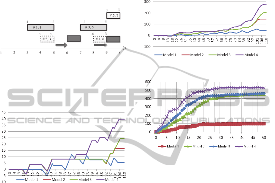
Figure 2 are shown with dark grey, when penalties
are applied; light grey marks orders without delay;
shifts in schedule are shown with wide arrows;
shifted orders are shown with dotted borders;
rejected order is white (not visible).
Figure 2: Diagram of execution of adaptive schedule by
one truck.
4 THE RESULTS OF THE
EXPERIMENTS
Figure 3: Dynamics of a profit for the truck depending on
model of transportation.
Trucks schedules were created for orders based on
the 4 used models of transportation. Graphs of
dynamic profit per each truck and dynamics of sum
of trucks profit depending on time was found
(Figure 3 – Figure 4). The designed MAS allows
also to study the profit depending on trucks number
for each flow of orders. For simplicity we don’t
consider standing costs of trucks. The trucks amount
was varied from 0 to 50 (Figure 5). Satiation modes
differ for the different models. The lowest profit
value is in the Model #1 because less amount of
orders are scheduled and additional expenses occur
after returning to the base. The Model #3 far exceeds
the Model #2 because it uses the same amount of
trucks as in Model #2 but more orders are scheduled.
But in a satiation mode it gives almost no benefits
vs. the Model #2, because when the trucks number is
high enough there are very few orders that are
executed with delays so Model #2 and Model #3 will
be almost equal. The Model #4 is the best one. It
gives approximate 20% more profit then Model #2
and Model #3. It allows using less trucks during the
plan execution. The reason is the adaptive re-
scheduling of orders in real time.
Figure 4: Dynamics of sum of trucks profit depending on
transportation models.
Figure 5: The dependence of the profit to the used trucks
number in the different transportation models.
REFERENCES
Leung , Y-T., 2004. Handbook of Scheduling: Algorithms,
Models and Performance Analysis. Chapman & Hall.
London.
Bonabeau, E., Theraulaz, G., 2000. Swarm Smarts. What
computers are learning from them? Scientific
American, vol. 282, no. 3, pp. 54-61.
Wooldridge, M., 2002. An Introduction to Multi-Agent
Systems. JohnWiley & Sons. London, 2
nd
edition.
Skobelev, P.: Multi-agent technology for real time
resource allocation, scheduling, optimization and
controlling in industrial applications, 2011. In
HoloMAS 2011, 5th International Confrence on
Industrial Applications of Holonic and Multi-Agent
Systems. Springer. Berlin. pp. 1-14.
Ivaschenko, A., Skobelev, P., Tsarev, A., 2011. ‘Smart
solutions’ multi-agent platform for dynamic
transportation scheduling. In ICAART 2011, 3rd
International Conference on Agents and Artificial
Intelligence, vol. 2, pp. 372-375.
ComparingAdaptiveandNon-adaptiveModelsofCargoTransportationinMulti-agentSystemforRealTimeTruck
Scheduling
285
