Contradiction Resolution for Foreign Exchange Rates Estimation

Ryotaro Kamimura

IT Education Center, 1117 Kitakaname, Hiratsuka, Kanagawa 259-1292, Japan

Keywords:

Self-evaluation, Outer-evaluation, Contradiction Resolution, Information-theoretic Learning, Free Energy,

SOM.

Abstract:

In this paper, we propose a new type of information-theoretic method called ”contradiction resolution.” In this

method, we suppose that a neuron should be evaluated for itself (self-evaluation) and by all the other neurons

(outer-evaluation). If some difference or contradiction between two types of evaluation can be found, the

contradiction should be decreased as much as possible. We applied the method to the self-organizing maps

with an output layer, which is a kind of combination of the self-organizing maps with the RBF networks. When

the method was applied to the dollar-yen exchange rates, prediction and visualization performance could be

improved simultaneously.

1 INTRODUCTION

In this paper, we propose a new information-theoretic

method called ”contradiction resolution,” aiming to

improve prediction and visualization performance. In

the method, a neuron is evaluated differently. If con-

tradiction between different types of evaluation can

be observed, this contradiction is decreased as much

as possible. We here consider only two types of eval-

uation, namely, self and outer-evaluation. In the self-

evaluation, a neuron’s output is evaluated for itself,

meaning that the output is determined by consider-

ing the neuron itself. On the other hand, in the outer-

evaluation, a neuron’s output is evaluated by consid-

ering all possible neighboring neurons. Then, if the

outputs from the self and outer-evaluation are differ-

ent from each other, this difference or contradiction

should be minimized.

In neural networks, no attempts have been made to

consider different types of evaluation. Some methods

have been exclusively concerned with self-evaluation.

More concretely, neurons have been forced to be as

independent as possible (Comon, 1994). On the other

hand, neurons have been forced to cooperate with

each other as much as possible in the self-organizing

maps (Kohonen, 1995), (Kohonen, 1990), (Kohonen,

1982). In the self-organizing maps, much attention

has been paid to the outer-evaluation for coopera-

tion. In our method, we can separate self and outer-

evaluation, meaning that we can examine the inﬂu-

ence of the other neurons on a neuron. Then, we can

control this inﬂuence depending upon given objec-

tives. In this paper, we aim to improve prediction as

well as visualization performance. This improvement

is expected to be realized only when we can ﬂexibly

control self and outer-evaluation.

2 THEORY AND

COMPUTATIONAL METHODS

2.1 Self and Outer Evaluation

We distinguish between self- and outer-evaluation

for neurons. Figure 1(a) shows an example of self-

evaluation, where a neuron in the center produces its

output, independently of its neighbors. This is called

”self-evaluation,” because the output can be obtained

only by evaluating its own activity. In other words,

neurons respond to input patterns individually. A self-

evaluated neuron responds to input patterns without

considering the outputs of the neighboring neurons.

On the other hand, a neuron’s output is determined by

considering all neighboring neurons except the neu-

ron itself, as shown in Figure 1(b). Thus, the neu-

ron’s output is determined by evaluating all neighbor-

ing neurons’ outputs except the output from the neu-

ron itself. This situation is called ”outer-evaluation.”

529

Kamimura R..

Contradiction Resolution for Foreign Exchange Rates Estimation.

DOI: 10.5220/0004152905290535

In Proceedings of the 4th International Joint Conference on Computational Intelligence (NCTA-2012), pages 529-535

ISBN: 978-989-8565-33-4

 2012 SCITEPRESS (Science and Technology Publications, Lda.)

Competitive unit

p(j|s)

q(j|s)



(a) Self-evaluation

Competitive units

(b) Outer-evaluation

Figure 1: Two types of evaluation, namely, self (a) and outer (b) evaluation.

2.2 Self and Outer-evaluated Outputs

Let us explain how to compute outputs by self and

outer-evaluation shown in Figure 1. The jth competi-

tive unit output can be computed by

= exp



−

− c

)

− c

)



, (1)

where x

and c

are supposed to represent L-

dimensional input and weight column vectors, where

L denotes the number of input units. The L×L matrix

is called a ”scaling matrix,” and the klth element of

the matrix denoted by ( )

is deﬁned by

(

)

= δ

, k, l = 1, 2, · ·· , L. (2)

where σ

is a spread parameter. In our experiments,

the spread parameter is computed by

, (3)

where β is larger than zero. The output is increased

when connection weights become closer to input pat-

terns. Now, suppose that the jth neuron is related to

the mth neuron by φ

. In order to demonstrate how

our method of contradiction resolution can be used,

we applied them to self-organizing maps. For this ap-

plication, all we have to do is to replace the relation

function φ

by the SOM’s neighborhood function.

The neighborhood function is deﬁned by

∝ exp

− r

2σ

, (4)

where r

and r

denote the position of the jth and

the cth unit on the output space, and σ

is a spread

parameter.

Then, the output from the jth neuron by the self-

evaluation is deﬁned by

∑

m=1

, (5)

where M is the number of competitive units and δ

is one only if j = m, and zero for all the other cases.

Thus, the output y

is equivalent to the output v

. The

normalized output can be deﬁned

p( j | s) =

∑

m=1

. (6)

Then, we consider outer-evaluation, which is deﬁned

∑

m=1

(1− δ

)φ

. (7)

IJCCI2012-InternationalJointConferenceonComputationalIntelligence

530

The output by the outer-evaluation is the sum of all

neighboring neurons’ outputs except the jth neuron.

The normalized output is deﬁned by

q( j | s) =

∑

m=1

. (8)

2.3 Contradiction Resolution

Our objective is to minimize contradiction between

the self- and outer-evaluation. To represent the con-

tradiction, we introduce the Kullback-Leibler diver-

gence between two types of neurons

KL =

∑

s=1

p(s)

∑

j=1

p( j | s)log

p( j | s)

q( j | s)

, (9)

where S is the number of input patterns. When the

KL divergence is minimized, supposing that errors

between patterns and weights are ﬁxed, we have

∗

( j | s) =

q( j | s)v

∑

m=1

q(m | s)v

. (10)

By puting this optimal ﬁring probability into the KL

divergence, we have the free energy function:

F = −2σ

∑

s=1

p(s)

×log

∑

j=1

exp



−

− c

)

− c

)



(11)

This equation can be expanded as

F =

∑

s=1

p(s)

∑

j=1

p( j | s)kx

− w

+2σ

∑

s=1

p(s)

∑

j=1

p( j | s)log

p( j | s)

q( j | s)

(12)

Thus, the free energy can be used to decrease KL di-

vergence as well as quantization errors. By differenti-

ating the free energy, we can realize the re-estimation

formula

∑

s=1

∗

( j | s)x

∑

s=1

∗

( j | s)

. (13)

3 RESULTS AND DISCUSSION

In computing the experimental results, attention was

paid to the easy reproduction and evaluation of the

ﬁnal results. For easy reproduction, we used the

well-known SOM toolbox of Vesanto et al. (Vesanto

et al., 2000) because the ﬁnal results of the SOM have

been very different, given the small changes in im-

plementation such as initial conditions. We have con-

ﬁrmed the reproduction of stable ﬁnal results by using

this package. In addition, we used the RBF network

learning to obtain connection weight from competi-

tive units to output units without any regularization

terms, because we did not obtain favorable results by

using the regularization. For comparison, we used the

results by the conventional RBF networks in which

regularization parameters were controlled to produce

the best possible results.

3.1 Dollar-Yen Exchange Rates

We used the dollar-yen exchange rate ﬂuctuation of

2011 for the purpose of visualization and prediction.

The two-thirds of the data were used for training and

the remaining data was for testing. We tried to exam-

ine how the prediction and visualization performance

could be improved. For example, in terms of visual

performance, we tried to extract features we could

intuitively infer from the exchange rates. Figure 2

shows the exchange rates during 2011. The period

was divided into three main periods, with an addi-

tional one showing the highest and lowest peaks. In

the ﬁrst period, relatively high rates are observed. Be-

tween the ﬁrst and the second period, the rates ﬂuc-

tuated greatly, reaching the highest and lowest points.

In the second period, the rates gradually decreased.

Finally, in the third period, the rates became lowerand

more stable. We must examine how our intuition for

the exchange rates can be realized by the conventional

self-organizing maps and contradiction resolution.

3.1.1 Prediction Performance

First, we examined how our method could improve

prediction performance for the testing and training

data. Table 1 shows the summary of errors and in-

formation when the map size is 10 by 5. The mean

squared errors between outputs and targets for the

testing data were 0.240 when the parameter β was

one. Then the errors decreased gradually and reached

their lowest point of 0.054 when the parameter β was

ten. On the other hand, by the conventional SOM and

the RBF with the Ridge regression, the errors were

0.056 and 0.062, respectively. Thus, the contradiction

resolution showed the lowest errors for the MSE. Cor-

relation coefﬁcient between targets and outputs in-

creased gradually from 0.736 (β = 1) to the lowest

of 0.933 (β = 10). On other hand, the SOM and RBF

produced 0.929 and 0.919, respectively. The correla-

ContradictionResolutionforForeignExchangeRatesEstimation

531

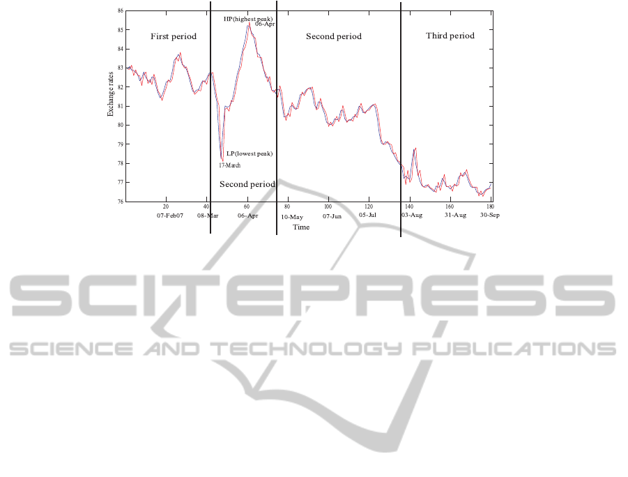
Figure 2: Training data of dollar-yen exchange rates during 2011.

tion coefﬁcient by the contradiction was higher than

that by the conventional two methods.

Then, we computed quantization and topographic

errors for the training data. The quantization errors

decreased gradually and reached the ﬁnal point of

0.437 when the spread parameter β was increased

from one to 20. By the conventional SOM, the quan-

tizatoin error was 0.505. The topographic error in-

creased from zero ((β = 1) to the maximum value

of 0.206 (β = 10). Then, the topographic error de-

creased gradually and reached the lowest point of

0.039. The topographic error by the SOM was 0.211.

Finally, mutual information between input patterns

and competitive units increased gradually when the

parameter β was increased. We could see that the

correlation coefﬁcient between information and MSE

was -0.947. When information increased, the MSE

between outputs and targets for the testing data de-

creased. The correlation coefﬁcient between infor-

mation and the coefﬁcient coefﬁcient between outputs

and targets was 0.874. When mutual information be-

tween input patterns and competitive units increased,

the correlation coefﬁcient between outputs and targets

increased. We could also see that the correlation co-

efﬁcient between information and quantization errors

was -0.992, meaning that quantization errors decease

when mutual information or organization increased.

This means that mutual information increase or in-

crease in organization in networks is closely related

to prediction and visualization performance except to-

pographic errors.

3.1.2 Visual Performance

Figure 3 shows the U-matrices by SOM and our

method. Figure 3 (a) shows the U-matrix by the con-

ventional SOM where we could not see clear class

boundaries. On the other hand, when the parame-

ter β was three in Figure 3(b), one straight bound-

ary in brown could be detected in the middle of

the U-matrix. When the parameter was increased to

ﬁve in Figure 3(c), the straight boundary deteriorated

slightly on the right hand side of the line. When the

parameter was further increase from 10 in Figure 3(d)

to 20 in Figure 3(f), class boundaries in warmer colors

became more complicated. Figures 4(a) and (b) show

the U-matrices and the corresponding labels by the

conventional SOM (b) and by the contradiction reso-

lution (a) when the network size was 10 by 5 and the

parameter β was ten. We can infer from these ﬁgures

that the entire period was divided into three periods,

namely, ﬁrst, second and third period. In addition, the

highest and lowest peaks were separately treated as

shown in Figure 2(a). On the other hand, by the con-

ventional SOM in Figure 2(b), class boundaries on the

U-matrix and the labels were weaker.

3.2 Discussion

We here discuss visual and prediction performance

with some remarks on the possibility of our method.

First, our method could be applied to the self-

organizing maps to improve visualization perfor-

mance. In self-organizing maps, neurons are treated

equally, having no individual characteristics. The

main objective is to make neurons as similar as possi-

ble to each other. The self-organizing maps’ property

of cooperation has the effect to weaken class bound-

aries. Thus, many methods on the visualization of

SOM knowledge have been accumulated (Sammon,

1969), (Ultsch and Siemon, 1990), (Ultsch, 2003),

(Vesanto, 1999), (Kaski et al., 1998), (Yin, 2002), (Su

and Chang, 2001), (Xu et al., 2010), to cite a few. Our

contradiction resolution, as shown in the experimen-

IJCCI2012-InternationalJointConferenceonComputationalIntelligence

532

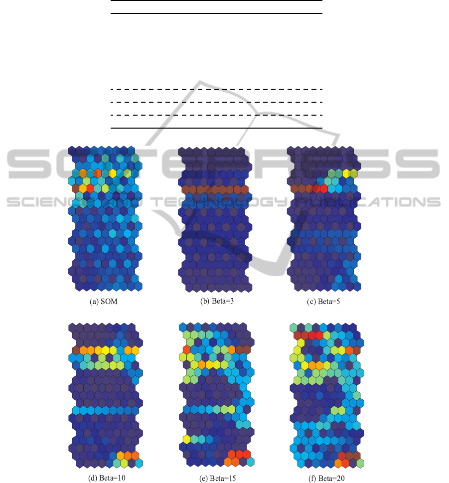
Table 1: MSE between outputs and targets, correlation coefﬁcient (CC) between outputs and targets, quantization errors (QE),

topographic errors (TE) and mutual information by our method and SOM for 10 by 5 map. The symbol CC

∗

represents

correlation coefﬁcients between information (INF) and the other measures. The symbol RR represents the RBF networks

with Ridge regression.

β MSE CC QE TE INF

1 0.240 0.736 3.960 0.000 0.000

3 0.068 0.914 0.999 0.100 0.117

5 0.072 0.908 0.670 0.200 0.129

10 0.054 0.933 0.581 0.206 0.130

15 0.055 0.932 0.504 0.072 0.132

20 0.055 0.932 0.437 0.039 0.135

SOM 0.056 0.929 0.505 0.211 0.134

∗

-0.947 0.874 -0.992 0.255

RR 0.062 0.919

Figure 3: U-matrices by the conventional SOM (a) and our method with 10 by 5 map whose parameter β ranged between 3

an 20 for the dollar-yen exchange rate.

tal results, can control cooperation so as to minimize

contradiction between individual and collective char-

acteristics of neurons. Experimental results showed

that this control of cooperation was effective in pro-

ducing produce clearer class boundaries.

Second, our method could improve prediction per-

formance. Compared with the results by the RBF with

the Ridge regression, our method showed better per-

ContradictionResolutionforForeignExchangeRatesEstimation

533

Figure 4: U-matrix and labels for 10 by 5 map by contradiction resolution (a) and SOM (b) for the dollar-yen exchange rate.

formance in terms of MSE and correlation coefﬁcient

between outputs and targets for the testing data as in

Table 1. When visual performance, for example, in

terms of the U-matrix, was improved, prediction per-

formance seemed to be improved as in Table 1. In

neural learning, one of the most serious problems is

that we cannot interpret and explain why and how

neural networks can produce outputs. Internal repre-

sentations obtained by learning is so complex that it is

impossible to interpret them. In addition, we can say

that interpretation is not necessarily related to the im-

proved prediction performance. We must improve the

prediction performance, scarifying interpretation per-

formance. The present results suggest that prediction

and interpretation performance are closely related and

both types of performance can be improved simulta-

neously.

Finally, contradiction resolution can be extended

to a variety of relations between neurons. Because we

used self-organizing maps, relations between neurons

were estimated by distance between neurons on the

map. However, we can imagine a variety of relations

between neurons. One possibility is that even if two

neurons are far from each other in terms of distance

on the map, they can be considered to be close to each

other if they respond quite similarly to input patterns.

By incorporating different types of relations between

neurons, we can create different types of neural net-

work for different objectives.

IJCCI2012-InternationalJointConferenceonComputationalIntelligence

534

4 CONCLUSIONS

In this paper, we have proposed a new type of

information-theoretic method called ”contradiction

resolution.” In this method, a neuron is evaluated for

itself (self-evaluation) and by all the other neurons

(outer-evaluation). If some difference or contradic-

tion between two types of evaluation can be found, it

should be decreased as much as possible. We applied

the method to the dollar-yen exchange rate ﬂuctua-

tion. Our method showed better performance in terms

of visualization and prediction performance. For ex-

ample, the prediction performance for the testing data

was better than that by the conventional SOM and the

RBF with ridge regression. The U-matrices obtained

by our method showed much clearer class boundaries

by which we could classify the dollar-yen exchange

rates into three periods. In addition, quantization and

topographic errors could be decreased to a level lower

than that by the conventional SOM. This means that

the prediction performance could be improved, keep-

ing ﬁdelity to input patterns. Thus, our method shows

a possibility that prediction performance and visual-

ization performance can be improved simultaneously.

REFERENCES

Comon, P. (1994). Independent component analysis: a new

concept. Signal Processing, 36:287–314.

Kaski, S., Nikkila, J., and Kohonen, T. (1998). Methods

for interpreting a self-organized map in data analysis.

In Proceedings of European Symposium on Artiﬁcial

Neural Networks, Bruges, Belgium.

Kohonen, T. (1982). Self-organized formation of topo-

logical correct feature maps. Biological Cybernetics,

43:59–69.

Kohonen, T. (1990). The self-organization map. Proceed-

ings of the IEEE, 78(9):1464–1480.

Kohonen, T. (1995). Self-Organizing Maps. Springer-

Verlag.

Sammon, J. W. (1969). A nonlinear mapping for data struc-

ture analysis. IEEE Transactions on Computers, C-

18(5):401–409.

Su, M.-C. and Chang, H.-T. (2001). A new model of self-

organizing neural networks and its application in data

projection. IEEE Transactions on Neural Networks,

123(1):153–158.

Ultsch, A. (2003). U*-matrix: a tool to visualize clusters in

high dimensional data. Technical Report 36, Depart-

ment of Computer Science, University of Marburg.

Ultsch, A. and Siemon, H. P. (1990). Kohonen self-

organization feature maps for exploratory data anal-

ysis. In Proceedings of International Neural Network

Conference, pages 305–308, Dordrecht. Kulwer Aca-

demic Publisher.

Vesanto, J. (1999). SOM-based data visualization methods.

Intelligent Data Analysis, 3:111–126.

Vesanto, J., Himberg, J., Alhoniemi, E., and Parhankan-

gas, J. (2000). SOM toolbox for Matlab. Technical

report, Laboratory of Computer and Information Sci-

ence, Helsinki University of Technology.

Xu, L., Xu, Y., and Chow, T. W. (2010). PolSOM-a new

method for multidimentional data visualization. Pat-

tern Recognition, 43:1668–1675.

Yin, H. (2002). ViSOM-a novel method for multivari-

ate data projection and structure visualization. IEEE

Transactions on Neural Networks, 13(1):237–243.

ContradictionResolutionforForeignExchangeRatesEstimation

535