
BINGR: Binary Search based Gaussian Regression
Harshit Dubey, Saket Bharambe and Vikram Pudi
International Institute of Information Technology - Hyderabad, Hyderabad, India
Keywords:
Regression, Gaussian, Prediction, Logarithmic Performance, Linear Performance, Binary Search.
Abstract:
Regression is the study of functional dependency of one variable with respect to other variables. In this paper
we propose a novel regression algorithm, BINGR, for predicting dependent variable, having the advantage of
low computational complexity. The algorithm is interesting because instead of directly predicting the value
of the response variable, it recursively narrows down the range in which response variable lies. BINGR
reduces the computation order to logarithmic which is much better than that of existing standard algorithms.
As BINGR is parameterless, it can be employed by any naive user. Our experimental study shows that our
technique is as accurate as the state of the art, and faster by an order of magnitude.
1 INTRODUCTION
The problem of regression is to estimate the value of
dependent variable based on values of one or more
independent variables, e.g., predicting price increase
based-on demand or money supply based-on inflation
rate etc. Regression analysis is used to understand
which among the independent variables are related
to the dependent variable and to explore the forms
of these relationships. Regression algorithms can be
used for prediction (including forecasting of time-
series data), inference, hypothesis-testing and mod-
eling of causal relationships.
Statistical approaches try to learn a probability
function P(y | x) and use it to predict the value of y
for a given value of x. Users study the application do-
main to understand the form of this probability func-
tion. The function may have multiple parameters and
coefficients in its expansion. Generally, these parame-
ters and coefficients have to be learned from the given
data, so as to give the best fit for the available data.
The existing standard algorithms (Desai et al.,
2010; Han and Kamber, 2000; L. Breiman and Stone,
1999) suffer from one or more of high computational
complexity, poor results, selection of parameters and
extensive memory requirements e.g. KNN (Han and
Kamber, 2000) gives accurate results but at the cost
of high computational complexity, Decision trees (L.
Breiman and Stone, 1999) can become too complex
and memory extensive, etc.
This motivated us to strive for an algorithm which
has low computational complexity, is simple, gives
accurate results and is parameterless. Our main con-
tribution, in this work, is a new regression algorithm
Binary search based Gaussian Regression (BINGR).
Our proposed algorithm gives accurate results in log-
arithmic time which is a significant improvement over
the existing linear time regression algorithms. Also,
our algorithm is parameterless and does not require
any knowledge of the domain in which it is to be ap-
plied.
Before presenting the algorithm, we would like to
mention some of its salient features. BINGR is highly
efficient with computational complexity of O(logn)
as compared to O(n) of other existing standard algo-
rithms, where n is the number of tuples present in
dataset. The algorithm is also parameterless, accu-
rate, generic and highly efficient. It is also simple to
understand and easy to implement.
In our algorithm, we don’t predict the values of
response variable directly. Instead we try to mini-
mize the range in which the response variable has the
maximum probability of occurrence. Also, the algo-
rithm presented does not require any prior study of the
dataset, to set any of the parameters or coefficients.
Hence the algorithm can be employed by any naive
user.
To get a precise and better understanding, it is im-
portant to formulate the problem as a mathematical
model. We do this in the next section.
2 PROBLEM FORMULATION
In this section, we present the mathematical model
258
Dubey H., Bharambe S. and Pudi V..
BINGR: Binary Search based Gaussian Regression.
DOI: 10.5220/0004159302580263
In Proceedings of the International Conference on Knowledge Discovery and Information Retrieval (KDIR-2012), pages 258-263
ISBN: 978-989-8565-29-7
Copyright
c
2012 SCITEPRESS (Science and Technology Publications, Lda.)

used to model the dataset and state the assumption
along with their justification.
The problem of regression is to estimate the value
of a dependent variable (known as response variable)
based on values of one or more independent variables
(known as feature variables). We model the tuple as
{X, y} where X is an ordered set of variables (prop-
erties) like {x
1
, x
2
, ..., x
n
} and y is the variable to be
predicted. Here x
i
are variables.
Formally, the problem has the following inputs:
• An ordered set of feature variables X ie {x
1
, x
2
,
..., x
n
}
• A set of tuples called the training dataset, D, =
{(X
1
, y
1
), (X
2
, y
2
), .. ., (X
m
, y
m
)}.
The output is an estimated value of y for the given X.
Mathematically, it can be represented as
y = f(X,D, parameters), (1)
where parameters are the arguments which the func-
tion f() takes. These are generally set by user and are
learned by trial and error method.
We assume that the dependent variable is only
dependent on the independent variables and nothing
else. This is the sole assumption we make. If this as-
sumption is not satisfied, then there is no chance of
obtaining accurate estimates even with the best pos-
sible regression algorithms available. In the coming
section we discuss work done related to this topic.
3 RELATED WORK
Before presenting our algorithms, we would like to
throw light on related work done in the recent past
The most common statistical regression approach
is linear regression (Seber and Lee, 1999) which as-
sumes the entire data to follow a linear relationship
between the response variable and the feature vari-
ables. Linear Regression does not perform well if the
relationship between the variables is not linear.
One of the widely used regression algorithm is
KNN i.e. K-Nearest-Neighbors. In this algorithm dis-
tance of the test tuple is calculated from every train-
ing tuple, and output is given based on the k near-
est tuples. It is resistant to outliers. There is no
pre-processing; every calculation is done in run-time.
Hence it has high computation complexity and per-
forms poorly as far as efficiency is concerned. More-
over, it requires learning of a parameter; asking the
user to have some understanding of the domain.
Another class of regression algorithms is SVM
(Smola and Scholkopf, 1998), Support Vector Ma-
chines. Support Vector Machines are very specific
class of algorithms, characterized by usage of kernels,
absence of local minima, sparseness of the solution
and capacity control obtained by acting on the margin,
or on number of support vectors. SVM try to linearly
separate the dataset and use this technique for predic-
tion. SVM suffer several disadvantages like choice of
kernel, discrete data, multi-class classifiers, selection
of kernel function parameters, high algorithmic com-
plexity, extensive memory requirements etc.
Another popular class of regression algorithms is
Decision trees. These algorithms build up a tree,
which is later used for decision making. They gener-
ally don’t require any data cleaning. Since the prob-
lem of constructing an optimal decision tree is NP-
Complete, heuristic algorithms are used which take
locally optimal decisions. One of the major problems
with Decision trees is that the tree can become too big
and complex.
Neural networks (Haykin, 2009) are another class
of data mining approaches that have been applied for
regression. However, neural networks are complex
closed box models and hence an in-depth analysis
of the results obtained is not possible. Data min-
ing applications typically demand an open-box model
where the prediction can be explained to the user,
since it is to be used for his decision support.
One of the latest works in the field of regres-
sion is PAGER (Desai et al., 2010). Being derived
from nearest neighbor methods, PAGER is simple and
also outliers-resilient. It assigns weight to non-feature
variables based on how much they influence the value
of the response variable. But as it is derived from
KNN, it also suffers from poor run-time performance.
Our work shares resemblance with segmented or
piecewise regression (H.P.Ritzema, 1994). However
upon analysis, the techniques are entirely different. In
segmented regression the independent variables are
partitioned into segments. In our method, the re-
sponse variable is partitioned into two groups to fa-
cilitate a binary search based methodology.
Our work seems to share a resemblance with Bi-
nary logistic regression (Hilbe and Joseph, 2009).
However the technique is again entirely different. In
Binary logistic regression the response variable is as-
sumed to follow a binomial logit model and the pa-
rameters of this model are learnt from training data.
4 BINGR
In this section we present the BINGR Algorithm, fol-
lowed by experimental results in the next section. The
algorithm is straightforward and follows the Divide
and Conquer kind-of policy.
BINGR:BinarySearchbasedGaussianRegression
259

The pre-processing of the algorithm is to sort the
training data tuples on basis on increasing value of y-
attribute. Sorting can be either ways (increasing or de-
creasing), it is just that we preferred increasing value
of y-attribute. This is the only pre-processing step re-
quired.
Let us consider the pseudo-code (Algorithm 1) of
BINGR algorithm. When a query comes, the train-
ing data is split into two parts (as shown in lines 2, 3
and 4). For splitting, the length of
half
1
is calculated
as total length divided by 2. Division is analogous to
integer division ie 6/2 = 3,7/2 = 3,8/2 = 4,9/2 =
4,10/2= 5 etc. The first
half len
tuples of the train-
ing dataset are put into
half
1
while rest are put into
half
2
.
Algorithm 1: Pseudo code of BINGR.
1: while len(training data) > 2 do
2: hal f len ←len(training data)/2
3: hal f
1
←training data[0,. . .,hal f len]
4: hal f
2
←training data[hal f len+ 1,...,]
5: P
1
← getGaussianProbability(query,hal f
1
);
6: P
2
← getGaussianProbability(query,hal f
2
);
7: if P
1
> P
2
then
8: training data ←hal f
1
9: else
10: training data ← hal f
2
11: end if
12: if min(p
1
/p
2
, p
2
/p
1
) ε [0.95, ... , 1.0] then
13: break from the loop.
14: end if
15: end while
16: print mean(y values in training data)
The next task is to find the probability of the query
belonging to those halves. This can be accomplished
by assuming Gaussian distribution of each indepen-
dent variable, for the half, estimating mean and vari-
ance using the Maximum Likelihood Estimate (Duda
and Stork, 2000) and then using the probability den-
sity function of Gaussian distribution (Equation 2).
1
√
2πσ
2
·e
−
(x−µ)
2
2σ
2
(2)
The probability of the query belonging to a half is
the product of probabilities of the independent vari-
ables belonging to that half. We take product because
the variables are assumed to be independent.
The half, having higher probability of query be-
longing to it, is now considered as the training dataset
and whole procedure is repeated again and again until
the breaking condition (line no 12) is met or length of
training dataset becomes sufficiently small (less than
2). Once achieved, the mean of the y-attributes in
training data
is quoted as output.
Sometimes, the probability of occurrence of query
in both the halves becomes nearly equal. In such
cases, a confident decision of assigning a half to
training data
can not be made. Hence, the break-
ing condition, i.e., if the ratio of probabilities lies be-
tween 0.95 and 1.0 then break the loop, is required.
The value of 0.95 was chosen after a lot experimenta-
tion on several datasets.
4.1 Complexity Analysis
It can be seen from Algorithm 1. that the while
loop iterates O(logn) times. Mean and variance for
partitions can be computed during the pre-processing
phase. Thus calculating probability of a query
belonging to a partition can be calculated in O(1)
computational time. The computational complexity
of the algorithm (apart from pre-processing) is, thus,
O(logn). KNN is linear in time, as for each query it
does a linear scan of the training data and then selects
the K nearest neighbors among them. We compare
the run-time of BINGR with KNN in Table 1.
Figure 1 shows a graphical comparison of the same.
The accuracy is discussed in the Experiments Section.
Table 1: Comparison of Run Times.
Number of Tuples BINGR KNN
10 94 72
100 452 507
1000 1685 5274
10000 2704 56283
100000 3575 549270
1000000 4281 5364766
Figure 1: Comparison of Run Times BINGR(red) and
KNN(green).
KDIR2012-InternationalConferenceonKnowledgeDiscoveryandInformationRetrieval
260

5 ILLUSTRATION
We will provide an illustration for a better understand-
ing of the algorithm. Consider the following dataset,
shown in Table 2.
Table 2: A Sample Dataset.
Tuple Number x
1
x
2
x
3
Y
1 24 32.9 29.2 18.7
2 24.5 32.1 28.6 18
3 23.4 32.5 29.8 17.4
4 23.2 32.4 29.7 19
5 23.2 31.8 29.7 18.3
6 24.1 32.9 29.8 18.8
7 23.9 31.4 29.9 18.9
8 23.6 32.7 29.9 19.1
9 23.2 32.1 29.3 18.5
10 23.5 32.6 28.8 18.3
11 23.8 32.1 29.6 18.8
And consider the tuple {23.7, 32.3, 28.9, 17.8}.
Here 17.8 is the actual answer while {23.7, 32.3,
28.9} is the query. The algorithm proceeds as de-
scribed below.
First the data is sorted on basis of increasing y-
value. The data is then divided into 2 halves; the first
one contains tuples numbered 1, 2,3, 4,and5 while
second half contains tuples numbered 6, 7, 8, 9, 10,
11. The probability of query belonging to first half
turns out to be 0.697 which is much greater than
that of second half i.e. 0.012. Also, the probabili-
ties are not similar, i.e., their ratio does not belong to
the range [0.95, ..., 1.0] and hence, we don’t break
from the loop. Thus, training data will now be the
first half. Length of training data, 5, is greater than
2 and hence the process will be repeated. The first
half now consists of tuples numbered 1 and 2 while
second half consists of tuples numbered 3, 4, and 5.
Again the probability of query belonging to first half
(0.792) turns out to be greater than that of second half
(0.039). Thus training data is assigned to first half.
Again, the probabilities are not similar (ratio = 0.049)
and hence, we continue with the loop. The length of
training data is equal to 2 and the average of y-values
{17.4, 18.0} in training data is quoted as output i.e.
17.7 which is a significantly accurate answer.
6 EXPERIMENTAL RESULTS
In this section we will compare our algorithm with
existing standard algorithms on standard datasets.
For comparing the results we have used two met-
rics, namely Absolute Mean Error (ABME) and Root
Mean Square Error (RSME). The datasets have been
taken from UCI data repository (uci, ), a brief de-
scription of the datasets follows later.
Absolute Mean Error (ABME) is the mean of ab-
solute difference of predicted value and the actual
value of dependent variable. Root Mean Square Error
(RMSE) is the square root of mean of squared differ-
ence of predicted value and actual value of the depen-
dent variable.
The performance of our algorithm has been eval-
uated against performance of widely known and used
regression algorithms namely, KNN (Han and Kam-
ber, 2000), Simple Linear (Seber and Lee, 1999),
RBF (Haykin, 2009) and LMS (Jung, 2005). These
algorithms were selected as they were shown to per-
form better than several other algorithms in a recent
study - PAGER (Desai et al., 2010). All results have
been obtained using leave one out comparison tech-
nique which is a specific case of n-folds cross valida-
tion (Duda and Stork, 2000) where n is set to number
of tuples in the dataset. The algorithms were simu-
lated on Weka (Hall and Ian, 2009) and best suited
parameter values were selected after trial and error
process. The parameter values have been summarized
in Table 3.
Table 4 and Table 5 illustrate the results of our
algorithm and their comparison with other standard
algorithms. Results in Table 4 (machine dataset and
autoprice dataset) show that our algorithms are most
suited to dense datasets, while Figure 2 and Figure 3
show graphical representation of results obtained on
Machine dataset and Housing Dataset respectively.
Table 3: Best Parameter values in Weka.
Algorithm Parameter Settings
Simple Linear Regression (Simple Linear Regres-
sion)
RBF Network (RBFNetwork -B 2 -S 1 -R
1.0E-8 -M -1 -W 0.1)
Least Median Square Re-
gression
(LeastMedSq -S 4 -G 0)
The CPU dataset (uci, ) has 6 independent vari-
ables and 1 dependent variable. The dataset consists
of 209 tuples.
The Housing dataset (uci, ) has 13 independent
variables and 1 dependent variable. It has 506 tuples.
The Housing dataset concerns housing values in sub-
urbs of Boston, which is the variable value to be pre-
dicted.
The Autoprice Dataset (mld, ) has 15 continu-
ous attributes, 1 integer attribute and 10 nominal at-
tributes, making a total of 26 attributes. The dataset
contains 206 tuples and is taken from mldata reposi-
tory (mld, ).
BINGR:BinarySearchbasedGaussianRegression
261
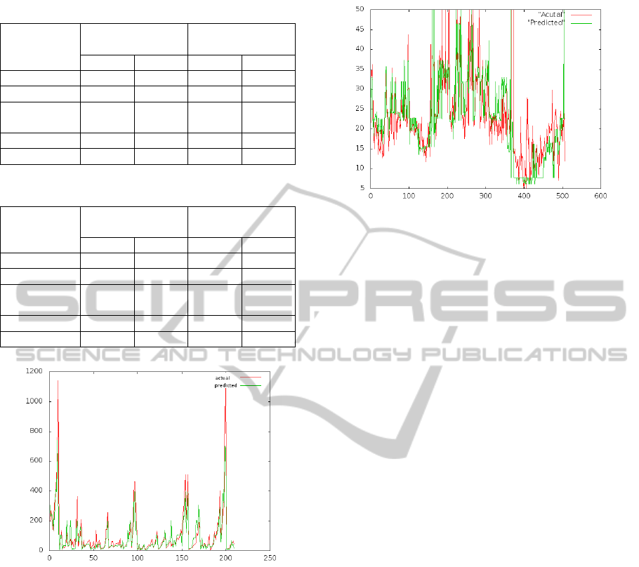
Table 4: Results on Machine and Autoprice Dataset.
Regression
Algorithms
Machine
Dataset
Autoprice
Dataset
AMBE RMSE AMBE RMSE
KNN 95 192 1609 2902
BINGR 36 78 1762 2735
Simple Lin-
ear
160 237 1906 2861
RBF 158 247 2751 4321
LMS 136 272 2211 3808
Table 5: Results on CPU and Housing Dataset.
Regression
Algorithms
CPU Dataset Housing
Dataset
AMBE RMSE AMBE RMSE
KNN 18.92 74.83 3.00 4.67
BINGR 25.55 75.34 4.7 6.81
Simple Lin-
ear
43.13 70.46 4.52 6.23
RBF 52.35 119.28 6.05 8.19
LMS 33.6 107.5 3.36 5.4
Figure 2: Results of BINGR on Machine Dataset, X axis
represent serial number of tuple. Y-axis represents value of
response variable.
The Machine dataset (uci, ) also has 6 indepen-
dent variables and 1 dependent variable. The dataset
consists of 209 tuples.
It can be seen that the algorithm is accurate
when compared to many existing standard algorithms.
Though KNN outperforms our algorithm in many
cases, taking linear time to compute the result, it is
important to note that it takes a parameter from the
user, demanding the user to have an understanding of
the domain. On the other hand, our algorithm pro-
vides quality results without asking for any parame-
ters from the user and that too in logarithmic time.
The main reasons for excellent performanceof our
algorithm are
• It recursivelynarrowdowns the range in which the
Figure 3: Results of BINGR on Housing Dataset, X axis
represent serial number of tuple. Y-axis represents value of
response variable.
expected value of the response variable lies.
• Our algorithm focuses on the local distribution
around the point for which the response variable
needs to be predicted.
7 CONCLUSIONS
In this paper we have presented a new regression al-
gorithm and evaluated it against existing standard al-
gorithms. The algorithm focuses on minimizing the
range in which the response attribute has the maxi-
mum likelihood. In addition to this, it does not re-
quire any understanding of the domain. As shown in
Complexity Analysis section, BINGR takes O(logn)
computation time, which is much better than the ex-
isting standard algorithms. Also the algorithm is sig-
nificantly more accurate than the existing state of art.
A lot of work is planned for enhancement of the
algorithm. For example, the value 4 in can be learned
from the dataset, i.e., there can be early break from
the while loop.
The output currently is quoted as mean of the y-
attribute values. This can be bettered by using some
interpolation method to give the output.
Also, studies can be carried out to find better split-
ting methods. For instance, splitting can be done con-
sidering values of y-attribute instead of simply bisect-
ing the dataset.
REFERENCES
Mldata repository, http://www.mldata.org.
Uci data repository, http://archive.ics.uci.edu.
Desai, A., Singh, H., and Pudi, V. (2010). Pager: Parameter-
less, accurate, generic, efficient knn-based regression.
KDIR2012-InternationalConferenceonKnowledgeDiscoveryandInformationRetrieval
262

Duda, R. O. and Stork, D. G. (2000). Pattern Classification
(2nd Edition). Wiley-Interscience.
Hall, M. and Ian, H. (2009). The weka data mining soft-
ware: An update. SIGKDD Explorations, 11.
Han, J. and Kamber, M. (2000). Data Mining: Concepts
and Techniques. Morgan Kaufmann Publishers.
Haykin, S. S. (2009). Neural networks: a comprehensive
foundation. Prentice Hall.
Hilbe and Joseph, M. (2009). Logistic Regression Models.
Chapman & Hall/CRC Press.
H. P. Ritzema (1994). Frequency and Regression Analysis.
Jung, K. M. (2005). Multivariate least-trimmed squares re-
gression estimato. Computational Statistics and Data
Analysis (CSDA).
L. Breiman and Stone, C. (1999). Classification and
Regression Trees. Monterey, CA: Wadsworth &
Brooks/Cole Advanced Books & Software.
Seber, G. A. F. and Lee, A. J. (1999). Linear Regression-
Analysis. Wiley Series in Probability and Statistics.
Smola, A. J. and Scholkopf, B. (1998). A tutorial on sup-
port vector regression. NeuroCOLT2 Technical Re-
portSeries.
BINGR:BinarySearchbasedGaussianRegression
263
