
4D Polygonal Approximation of the Skeleton for 3D Object
Decomposition
Luca Serino, Carlo Arcelli and Gabriella Sanniti di Baja
Institute of Cybernetics “E. Caianiello”, CNR, Naples, Italy
Keywords: 3D Object, Skeleton, Decomposition, Polygonal Approximation.
Abstract: We improve a method to decompose a 3D object into parts (called kernels, simple-regions and bumps)
starting from the partition of the distance labeled skeleton into components (called complex-sets, simple-
curves and single-points). In particular, each simple-curve of the partition is here interpreted as a curve in a
4D space, where the coordinates of each point are related to the three spatial coordinates of the
corresponding voxel of the 3D simple-curve and to its associated distance label. Then, a split type polygonal
approximation method is employed to subdivide, in the limits of the adopted tolerance, each curve in the 4D
space into straight-line segments. Vertices found in the 4D curve are used to identify corresponding vertices
in the 3D simple-curve. The skeleton partition is then used to recover the parts into which the object is
decomposed. Finally, region merging is taken into account to obtain a decomposition of the object more in
accordance with human intuition.
1 INTRODUCTION
Object decomposition is of interest to reduce the
complexity of computer vision tasks such as
description and recognition. The underlying theory
is that human object understanding is based on
recognition-by-component (Hoffman and Richards,
1984); (Singh et al., 1999).
Object decomposition can be achieved by
deriving information from a representation of the
object. If the surface delimiting a 3D object is used,
curvature variations along the object boundary can
be used to identify points through which surfaces,
separating different object parts, should pass
(Shamir, 2008); (Cheng et al., 2008). If the skeleton
is used, its geometrical structure can lead to the
identification of suitable skeleton subsets
corresponding to different parts of the object (de
Goes et al., 2008); (Macrini et al., 2008).
We favor the latter alternative and refer to the
skeleton denoted as curve skeleton in (Arcelli et al.,
2011). This is a subset of the 3D object, consists of
the curves symmetrically placed within the object
and has the same topology as the object. The
skeletonization method (Arcelli et al., 2011) is
related to the medial axis transform (Blum, 1973).
According to this model, the skeleton is the locus of
the symmetry points, i.e., the points of the object
that can be seen as centers of balls bi-tangent to the
object boundary and included in the object. Skeleton
points are labeled with the radii of the associated
balls, and the object can be recovered by the union
of the balls associated with the symmetry points.
The skeleton can be computed in the distance
transform of the object, where object voxels are
labeled with their distance from the complement of
the object. Each voxel can be interpreted as the
center of a ball with radius equal to the distance
label. A ball is maximal if is not included by any
other single ball in the object and its center is called
center of a maximal ball, CMB. The CMBs are
equidistant from at least two parts of the object's
boundary, hence they are symmetry points. Any ball
can be built by applying to its center the reverse
distance transformation (Borgefors, 1996). The
object can be recovered by applying the reverse
distance transformation to its CMBs.
Full object recovery from the skeleton is possible
only if the skeleton includes all the CMBs. This
happens only for objects consisting of parts with
tubular shape, where the CMBs are almost all
aligned along symmetry axes of the object.
However, the CMBs are generally placed along
symmetry planes and axes. Thus, to have a skeleton
consisting exclusively of curves, only a subset of the
CMBs can be included in the skeleton and full object
467
Serino L., Arcelli C. and Sanniti di Baja G. (2013).
4D Polygonal Approximation of the Skeleton for 3D Object Decomposition.
In Proceedings of the 2nd International Conference on Pattern Recognition Applications and Methods, pages 467-472
DOI: 10.5220/0004265204670472
Copyright
c
SciTePress
recovery is not guaranteed. This notwithstanding,
the skeleton has been profitably used for object
decomposition, whichever is the shape of the object.
In this paper, we present a decomposition
method based on skeleton partition and object
reconstruction, which is the follow up of a method
introduced in (Serino et al., 2010) and successively
improved in (Serino et al., 2011).
2 DECOMPOSITION SCHEME
We achieve object decomposition via the partition of
the distance labeled skeleton S. A key role is played
by the regions recovered by applying the reverse
distance transformation to the branch points of S,
i.e., to the skeleton voxels with more than two
neighboring skeleton voxels. For branch points
sufficiently close to each other, a single region is
obtain, which is called the zone of influence of the
branch points it includes. The zones of influence of
S allow us to group the branch points that for a
human observer correspond to a single branch point
configuration of an ideal skeleton representing the
object. The zones of influence are also used to
originate the partition of S. The components of the
skeleton partition are used as seeds to recover the
parts into which the object is decomposed.
2.1 Previous Work
The decomposition scheme (Serino et al., 2011)
splits 3D objects in perceptually significant non
overlapping parts by performing a partition of the
skeleton into at most three kinds of subsets (called
simple-curves, complex-sets, and single-points). See
Figure 1 left and middle left, showing the 3D object
horse and the partition of its skeleton into simple-
curves, green voxels, and complex-sets, red voxels.
Simple-curves, complex-sets, and single-points
were used to build respectively simple-regions,
bumps and kernels. Kernels are a sort of main bodies
of the object, from which simple-regions and bumps
protrude. Object parts were built in two steps. The
first step involves reverse distance transformation.
The second step performs an expansion with the aim
of assigning the object voxels not yet recovered by
the reverse distance transformation to the regions to
which they are closer. See Figure 1 middle right,
where kernels and simple regions for the horse are
shown in red and green, respectively.
A one-to-one correspondence exists between
partition components and object parts. However, in
some cases the number of parts may be not in
accordance with human intuition. For example,
some protrusions may be seen as negligible details
that do not deserve to be represented by individual
parts of the decomposition; similarly, two kernels
linked to each other by a simple-region may be
interpreted as constituting a unique main body, if the
linking simple-region is scarcely elongated. Thus, it
may be preferable to give up the one-to-one
correspondence and favor a decomposition more in
accordance with human perception. To this aim,
criteria for merging bumps and simple-regions to
their adjacent kernels were also suggested, so as to
obtain a decomposition of the object into a smaller
number of perceptually significant parts. See Figure
1 right, where the decomposition obtained after
merging is shown. The two kernels and the simple-
region in between them have been merged into a
unique component, the torso of the horse.
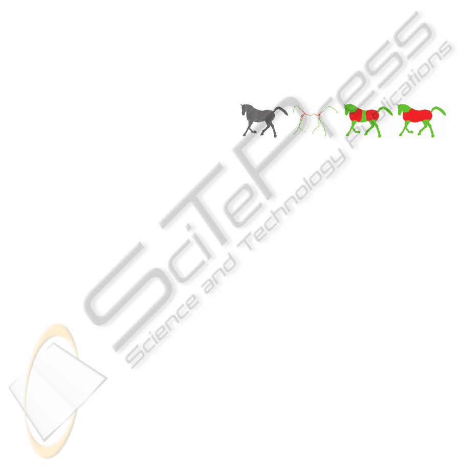
Figure 1: From left to right: the object horse; simple-
curves (green) and complex-sets (red) of the skeleton;
decomposition into kernels (red) and simple-regions
(green); decomposition after merging.
2.2 New Ideas
To our opinion, kernels and bumps are regions
whose description would not benefit of a further
subdivision into simpler parts. In fact, kernels are
almost convex bodies and bumps are elementary
protrusions. In turn, a simple-region, though having
the corresponding simple-curve as its unique
symmetry axis, may still be interpreted as having an
articulated structure. In fact, the surface separating a
simple-region from the complement of the object
may be characterized by curvature variations. In
addition, also the thickness of a simple-region,
measured in planes perpendicular to its associated
simple-curve, may significantly change. Thus, in this
paper we suggest an alternative decomposition
scheme that allows us to subdivide simple-regions
into smaller entities, called basic-regions, which are
characterized by absence of significant curvature
variations along the object boundary and by
thickness that is either nearly constant or evolves in
an almost monotonic manner.
We partition the skeleton as in (Serino et al.,
2011). Then, we divide the simple-curves into
segments, each of which consisting of voxels that
are aligned along straight lines and whose distance
values are either all equal or change in a monotonic
ICPRAM2013-InternationalConferenceonPatternRecognitionApplicationsandMethods
468
way. In fact, curvature changes along the boundary
of a simple-region are reflected by curvature
changes along its associated simple-curve. In turn,
thickness changes in a simple-region are reflected by
changes in the distance values of the voxels in the
associated simple-curve. Subdivision of each
simple-curve is obtained by resorting to polygonal
approximation in a 4D space, where any skeleton
voxel is mapped into a point whose coordinates are
related to the three Cartesian coordinates and the
distance value of the skeleton voxel. After all
simple-curves have been subdivided into straight-
line segments, we build the regions into which the
object is interpreted as decomposed. In particular,
regions corresponding to simple-curves will result to
be divided into a number of basic-regions, each of
which characterized by constant or monotonically
changing thickness and by absence of significant
curvature changes along the boundary.
3 THE METHOD
We use binary voxel images in cubic grids. The
333 neighborhood of a voxel p includes the six
face- the twelve edge- and the eight vertex-
neighbors of p.
The distance between two voxels p and q is the
length of a minimal path from p to q. If the weights
3, 4 and 5 suggested in (Borgefors, 1996) are used to
measure moves from p towards its face-, edge- and
vertex-neighbors along the path, the <3,4,5>-
distance is obtained.
The distance transform DT of an object P is a
multi-valued replica of P, where voxels are labeled
with their distance from the complement of P. We
compute DT by using the <3,4,5>-distance.
The k-th layer of DT is the set of voxels having a
distance value d such that (k-1)3<dk3 (Svensson
and Sanniti di Baja, 2002). Except for the first layer
that includes only voxels with distance label 3, any
other layer in DT includes voxels that are
characterized by up to three different values. The
value of a voxel p in the k-th layer depends on
whether its closest neighbors in the (k-1)-th layer,
i.e., the neighbors from which p received distance
information, are face-, edge- or vertex-neighbors of
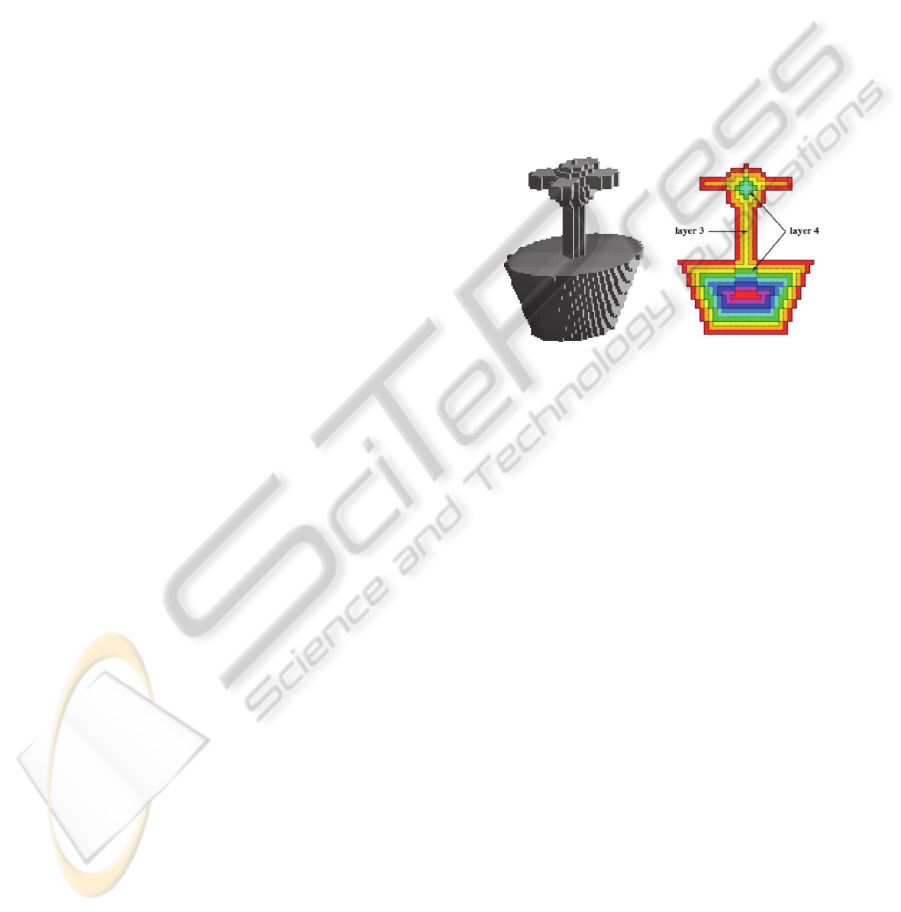
p. In Figure 2, a 3D object and a section of its
distance transform are shown, where the voxels
belonging to the same distance layer have been
colored with the same color.
The polygonal approximation of the simple-
curves in the partition of the skeleton S is computed
by using a split type algorithm (Ramer, 1972). Given
an open curve, the extremes of the curve are taken as
vertices of the polygonal approximation. To identify
the other vertices, we consider the straight line
joining the extremes of the curve and compute the
Euclidean distance from such a straight line of all
points of the curve; the point with the largest
distance is taken as a vertex if such a distance is
greater than an a priori fixed threshold (to be set
depending on the desired approximation quality).
Any detected vertex divides the curve into two
curves, to each of which the same splitting
procedure is applied. The splitting process is
repeated as far as points are detected having distance
larger than the threshold from the straight lines
joining the extremes of the curves to which the
points belong.
Figure 2: A 3D object, left, and a section of the <3,4,5>-
distance transform, right.
To perform polygonal approximation by taking
into account simultaneously changes in geometry
along the simple-curves and changes in distance
value of their voxels, we should represent the curves
in a 4D discrete space, where the coordinates are the
three Cartesian coordinates and the distance value of
the voxels of the 3D simple-curves. A simple-curve
in the 3D skeleton consists of voxels adjacent to
each other (each voxel has exactly two neighbors in
the curve, with the exception of the extremes of the
curve having only one neighbor), but may result in a
sparse set of points when passing to the 4D
representation. To have a connected set also in the
4D discrete space, we exploit the fact that the
algorithm (Arcelli et al., 2011) is based on the
<3,4,5> distance transform, where layers are easy to
detect, and adjacent skeleton voxels belong to the
same layer or to layers whose indexes differ by one.
Thus, we use the index of the layer to which a voxel
belongs in place of its distance as the 4th coordinate
of the corresponding point in the 4D space.
Given three points A, B and C in the 4D space,
the square of the Euclidean distance d of point C
from the straight line AB can be computed as:
d
2
= ||AC||
2
- P
ABC
* P
ABC
/ ||AB||
2
4DPolygonalApproximationoftheSkeletonfor3DObjectDecomposition
469

Figure 3: From top left to bottom right: an input object; its skeleton (different colors denote different distance labels);
vertices (black voxels) found on the skeleton by the 4D polygonal approximation; object decomposition.
where ||AB|| is the norm of the vector AB, and P
ABC
is the scalar product between vectors AB and AC.
Points with d> are taken as vertices of the
polygonal approximation. Once vertices have been
detected in the 4D space, we go back to the 3D
skeleton representation and mark the skeleton voxels
corresponding to the found vertices.
An example is given in Figure 3, showing an
input object, top left, and its skeleton, top right.
Different colors are used to show the different
distance labels of the skeleton voxels. Though the
skeleton is a straight-line segment in the 3D space,
its voxels have different distance labels due to the
fact that object thickness changes along the object.
The 4D polygonal approximation is applied to the
skeleton after the distance labels of the skeleton
voxels have been replaced by the layer indexes.
Vertices (black voxels in Figure 3 bottom left) are
found in the skeleton, which divide the skeleton into
four segments each of which corresponds to a
portion of the object characterized by monotonically
changing width (Figure 3 bottom right).
We have experimentally found that the threshold
value =20 is adequate to originate a polygonal
approximation sufficiently faithful to the original
curve and is, at the same time, able to prevent an
excessive fragmentation of the curve. Such a
threshold value has been used for the examples
shown in this paper as well as for all other objects
we have been working with. The vertices are shown
in black in Figure 4 top left for the running example.
The found vertices divide each simple-curve into a
number of consecutive segments, each of which
corresponding to a part of the simple-region
associated with the whole simple-curve, which is
characterized by absence of significant curvature
variations along the object boundary and by
thickness that is either nearly constant or evolves in
an almost monotonic manner.
Consecutive segments share a common vertex,
called hinge. We assign the same identity label to all
voxels in a segment, except for the hinges to which
we assign a unique identity label. The two extremes
of any simple-curve are ascribed the identity labels
of the two segments they belong to.
A process in two steps, following a strategy
similar to that suggested in (Serino et al., 2011), is
accomplished to build kernels, bumps and simple-
regions into which the object is decomposed.
Partition components are assigned identity labels
and are interpreted as seeds for region growing. In
the first step, the reverse distance transformation
with identity label propagation is applied to the
seeds. Care is taken to ascribe to the proper regions
the voxels that, being at the same distance from
different seeds, receive different identity labels and
to guarantee that the surfaces separating adjacent
regions are almost planar. The second step is done to
achieve complete recovery of the various regions,
since the skeleton of a 3D object generally does not
include all CMBs. Thus, object voxels that have not
been recovered by the reverse distance
transformation are assigned the identity label of the
region to which they result to be closer.
Since we aim at a decomposition where simple-
regions are articulated into basic-regions, during the
first step we propagate the labels assigned to the
segments and hinges identified by polygonal
approximation, rather than the labels ascribed to the
simple-curves. Voxels that can be recovered by
region growing applied to more than one
segment/hinge receive the unique special identity
label used for all hinges. Let us call hinge-regions
the connected components of recovered voxels with
the label of the hinges. Voxels of the hinge-regions
have to be re-distributed between the adjacent
regions. This is done during the second step by the
same process used to complete recovery of all
regions. Distance information is used to ascribe to
the voxels not recovered by reverse distance
transformation or belonging to hinge-regions the
identity label of the regions to which they are closer.
See Figure 4 top middle.
The final step of the process is devoted to
merging to the adjacent kernels those bumps and
simple regions that are perceived as not individually
meaningful.
A simple-region is considered as a whole for
merging, even if the region is articulated into basic-
regions. In fact, in our opinion the articulation of a
simple-region into basic-regions has to be taken into
account only to distinguish objects in the same class.
The relevance of a region R, considered for
merging to an adjacent kernel, is computed in terms
ICPRAM2013-InternationalConferenceonPatternRecognitionApplicationsandMethods
470
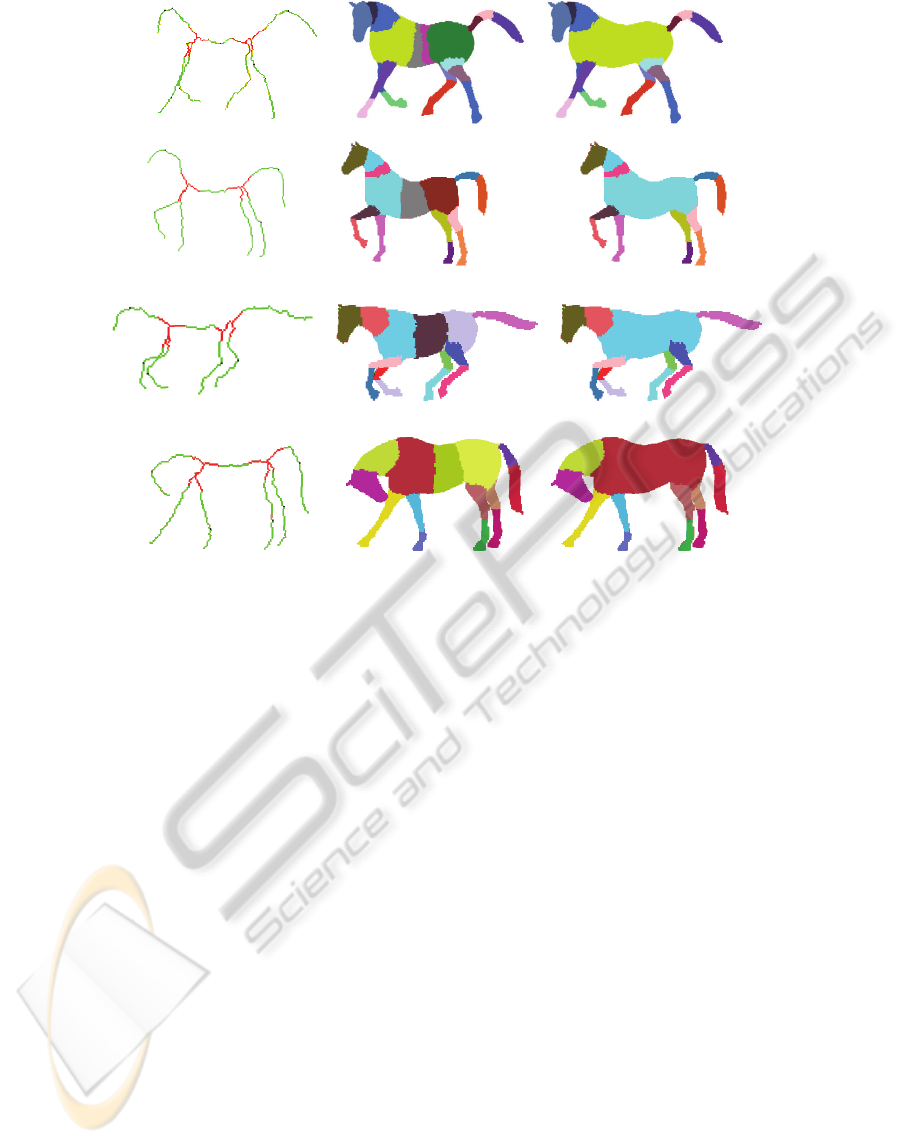
Figure 4: From left to right, skeleton partition (vertices of the polygonal approximation are in black), decomposition before
merging and decomposition after merging.
of two measures, as suggested in (Serino et al.,
2011). These are respectively the ratio between the
volume of R and the volume of the compound region
that would be obtained as result of merging, and the
ratio between the visible portion of the surface of R
(measured by the number of voxels in the surface of
R having at least one face-neighbor in the
background) and the non visible portion of the
surface of R (measured by the number of voxels in
the surface of R having at least one face-neighbor in
the adjacent kernels). Two thresholds, and , are
used for the above two ratios. In this work, the
values =1.2 and =2 have been used. For the
running example, the final decomposition is shown
in Figure 4 top right.
The decomposition after merging can be used to
identify the class to which an object belongs, in
terms of the number of kernels, bumps and simple-
regions, and of their spatial relationships. Moreover,
by taking into account the possibly existing basic-
regions, the decomposition can be used to
distinguish objects in the same class. If necessary,
the decomposition before merging can also be used
to derive information on the more or less articulated
structure into basic-regions of those simple-regions
that have been merged to the adjacent kernels. A few
examples for the object horse in different poses are
given in Figure 4.
The suggested method has been tested on several
3D images from publicly available shape
repositories, e.g., (Shilane et al., 2004), producing
generally satisfactory results. A few examples of the
performance of our method can be appreciated in
Figure 5.
4 CONCLUSIONS
A method to decompose a 3D object, starting from
the partition of its skeleton into complex-sets,
single-points and simple-curves, has been presented.
Simple-curves are interpreted as curves in the 4D
space, where the coordinates of each point are
computed in terms of the Cartesian coordinates and
the distance values associated to the skeleton voxels.
A polygonal approximation is done in the 4D
space to subdivide simple-curves into straight-line
segments. Straightness of segments regards both
geometric curvature along the 3D simple-curves and
distribution of distance values along the curves. The
same threshold value has been used for polygonal
approximation for all tested images. The elements of
the skeleton partition are used as seeds to
4DPolygonalApproximationoftheSkeletonfor3DObjectDecomposition
471
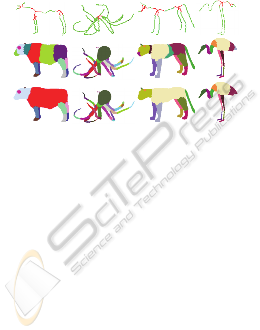
Figure 5: Skeleton partitions, where vertices found on the simple curves are shown in black, and corresponding
decompositions before and after merging.
recover the parts (kernels, bumps and simple-
regions) into which the object is decomposed.
Simple regions may be articulated into basic-
regions, due to the polygonal approximation done on
the simple-curves. Merging is also accomplished to
obtain a more stable final decomposition, whose
parts agree with human perception.
REFERENCES
C. Arcelli, G. Sanniti di Baja, L. Serino, 2011. Distance
driven skeletonization in voxel images, IEEE Trans.
PAMI, 33, 709-720.
H. Blum, 1973. Biological shape and visual science, J.
Theor. Biol., 38, 205-287.
G. Borgefors, 1996. On digital distance transform in three
dimensions, CVIU, 64, 368-376.
Z-Q. Cheng, B. Li, G. Dang, S-Y. Jin, 2008. Meaningful
Mesh Segmentation Guided by the 3D Short-Cut Rule,
Proc. AGMP 2008, LNCS 4975, 244-257, Springer.
F.de Goes, S. Goldenstein, L. Velho, 2008. A Hierarchical
Segmentation of Articulated Bodies, Computer
Graphics Forum, 27, 1349-1356.
D. D. Hoffman, W. A. Richards, 1984. Parts of
Recognition, Cognition, 18, 65-96.
D. Macrini, K. Siddiqi, S. Dickinson, 2008. From
Skeletons to Bone Graphs: Medial Abstraction for
Object Recognition, Proc. CVPR 2008, 1-8.
U. Ramer, 1972. An Iterative procedure for the polygonal
approximation of plane curves, CGIP, 1, 244-256.
L. Serino, G. Sanniti di Baja, C. Arcelli, 2010. Object
decomposition via curvilinear skeleton partition, Proc.
ICPR 2010, 4081-4084, IEEE CS Press.
L. Serino, G. Sanniti di Baja, C. Arcelli, 2011. “Using the
skeleton for 3D object decomposition”, in A. Heyden
and F. Kahl (Eds.): SCIA 2011, LNCS 6688, 447-456,
Springer.
A. Shamir, 2008. A Survey on Mesh Segmentation
Techniques, Computer Graphics Forum, 27, 1539-
1556.
P. Shilane, P. Min, M. Kazhdan, T. Funkhouser, 2004. The
Princeton Shape Benchmark, Shape Modeling
International, Genova, Italy.
M. Singh, G. D. Seyranian, D. D. Hoffman, 1999. Parsing
Silhouettes: the Short-Cut Rule,
Perception&Psychophysics, 61, 636-660.
S. Svensson, G. Sanniti di Baja, 2002. Using distance
transforms to decompose 3D discrete objects, IMAVIS,
20, 529-540.
ICPRAM2013-InternationalConferenceonPatternRecognitionApplicationsandMethods
472
