Cage-free Spatial Deformations

Angels Cerver

Alvar Vinacua and Pere Brunet

Departament de Llenguatges i Sistemes Inform

atics LSI, Universitat Polit

ecnica de Catalunya,

Campus Nord, 08034 Barcelona, Spain

Keywords:

Generalized Barycentric Coordinates, Cage, 3D Model Deformations.

Abstract:

We propose a new deformation scheme for polygonal meshes through generalized barycentric coordinates that

does not require any explicit cage deﬁnition. Our system infers the connectivity of the control points deﬁned

by the user and computes the coordinates using this structure. This allows the user to incrementally position

the control points (or delete them) wherever he considers more suitable. This freedom gives more control,

precision and locality to the deformation process.

1 INTRODUCTION AND

PREVIOUS WORK

Cage-based Deformation is a widely used spatial

model-deformation system. The geometric model to

be deformed is located inside a polyhedron (or a poly-

gon) called cage. The vertices of the cage are the con-

trol points Q of the deformation and the vertices p

of the model are deﬁned as a convex combination of

Q using a system of Generalized Barycentric Coordi-

nates (GBC) (see Equation 1).

p =

∑

(p), (1)

where i is the index of the corresponding control point

and α

(p) is the GBC of p w.r.t control point q

The overall deformation consists in two steps:

1. Preprocess step: given the cage, the GBC α

(p)

are computed and stored for each vertex p.

2. Deformation step: every time the control points

are modiﬁed, the model is recomputed (see Equa-

tion 2).

∑

(p) (2)

Barycentric Coordinates, as proposed by Mbius

(Mbius, 1827), allow to deﬁne a point p inside a sim-

plex w.r.t its vertices. However, the restriction over

the polytope structure has led to the rise of different

Generalized Barycentric Coordinates (GBC) systems

that try to extend the classic scheme to use it in more

general polygons and polyhedra.

Wachspress (Wachspress, 1975) and Meyer et al.

(Meyer et al., 2002) deﬁned GBC systems that work

over convex polygons.

It wasn’t until the deﬁnition of the Mean-Value

Coordinates (MVC) (Floater, 2003; Floater et al.,

2006) and MVC in 3D (Floater et al., 2005; Ju et al.,

2005) that a solution to compute the coordinates over

concave polygons and polyhedra was given. How-

ever, MVC give negative results if the point p lies

outside the polygon (polyhedron in 3D) or outside the

kernel of the concave ones. For this reason, Lipman

et al. (Lipman et al., 2007) deﬁned the Positive MVC

which guarantee the positivity of the coordinates over

any domain.

At 2007, Joshi et al. (Joshi et al., 2007) pre-

sented the Harmonic Coordinates (HC), which can

work over any kind of polygon and polyhedron (con-

vex and concave) but do not have a closed formula.

Lipman et al. (Lipman et al., 2008) deﬁned the

Green Coordinates (GC) that can be used over any

kind of polygon and polyhedron. GC use vertices and

normals of the cage to complete their convex combi-

nation (see Equation 3).

p =

∑

(p) +

∑

(p), (3)

where j is the index of the corresponding face (edge).

Using GC, Li et al. (Li et al., 2010) developed

a technique to allow local and smooth deformations

over a shape without any kind of cage around it.

The main contribution of our proposed algorithm

is the ability toperform real-time mesh deformations,

without therequirement of deﬁning explicit cages.

The deformation is performed through a novel

system ofGBC and the users can locate the control

111

Cerveró M., Vinacua À. and Brunet P..

Cage-free Spatial Deformations.

DOI: 10.5220/0004285201110114

In Proceedings of the International Conference on Computer Graphics Theory and Applications and International Conference on Information

Visualization Theory and Applications (GRAPP-2013), pages 111-114

ISBN: 978-989-8565-46-4

 2013 SCITEPRESS (Science and Technology Publications, Lda.)

Compute

Structure

Compute

Generalized

Barycentric

Coordinates

Control

Points’

Generalized

Barycentric

Coordinates

Add/Delete Control Points

User Input Preprocess

Deformation

Figure 1: Deformation algorithm pipeline with two-step preprocess.

points anywhere, to ensure precise deformation con-

tol. Moreover, they can be inserted and deleted at any

time during the deformation.

Anoverview of the algorithm is presented in Sec-

tion 2. Sections 3 and 4detail the preprocess which

builds the auxiliary list of convexpartitions and com-

putes the GBC. Finally, Section 5 discusses our re-

sults, whereas Section 6 is devoted to theconclusions

and future work.

2 OVERVIEW

As already mentioned, our main goal is to derive a de-

formation schemewhich only considers the distribu-

tion of the control points in thespace, with no imposed

connectivity. Users should havecomplete freedom in

placing control points anywhere in the region of the-

model, not having to deﬁne cages and their polyhe-

dral topologies.The proposed deformation algorithm

includes two preprocessing steps:

1. A static framework of convex polyhedra is auto-

matically computed from the set ofuser-deﬁned

control points.

2. For every vertex p of the polygonal mesh to be

deformed, itsGBC α

(p) are computed and stored.

During the deformation, Equation 2 is used to

update thelocation of the mesh vertices, similarly to

cage-based deformation systems.

Figure 1 shows the complete pipeline of our de-

formation scheme.

3 NESTED PARTITIONS

Once the user has deﬁned the control points in the

vicinity of the model, our system needs to automati-

cally deﬁne some kind of connectivity between them

to support the calculation of the coordinates. This

connectivity is done through two complete partitions

of the convex hull (CH) of these points into triangu-

lated convex polyhedra.

The ﬁrst partition that our method calculates is

the convex hull. Then, the second partition is built

adding, one by one, those control points laying into

the CH, respecting the order in which the user had de-

ﬁned them (from more general to more local impact).

The ﬁrst added point performs a complete convex par-

tition of the CH and for the rest of the points, the algo-

rithm ﬁnds the already computed convex that contains

this point and substitutes it by a convex partition of it.

See Algorithm 1 and Figure 2 for an overview of the

algorithm.

Algorithm 1: Layers.of.nested.partitions.

Require: The control points Q

Ensure: P is the set of partitions

CH = GetConvexHull(Q)

AddPartition(P, CH)

Qint = GetInteriorCPoints(CH, Q)

part = GetPartition(CH, Qint[0])

for i = 1 to size(Qint)

convex = GetConvexWithQ(part, Qint[i])

sub_part = GetPartition(convex, Qint[i])

RemoveConvex(part, convex)

AddConvexes(part, sub_part)

AddPartition(P, part)

return P

Partitions are simply computed by spliting the

convex to be partitioned into a set of tetrahedra. See

Algorithm 2 for the pseudocode of this algorithm.

Algorithm 2: Get.Partition.

Require: A Convex and a control point Qint[i]

Ensure: Partition is the partition of Convex

into tetrahedra w.r.t Qint[i]

for j = 0 to numFaces(Convex)

face = GetFace(Convex, j)

tetra = GetTetrahedron(face, Qint[i])

AddTetrahedron(Partition, tetra)

return Partition

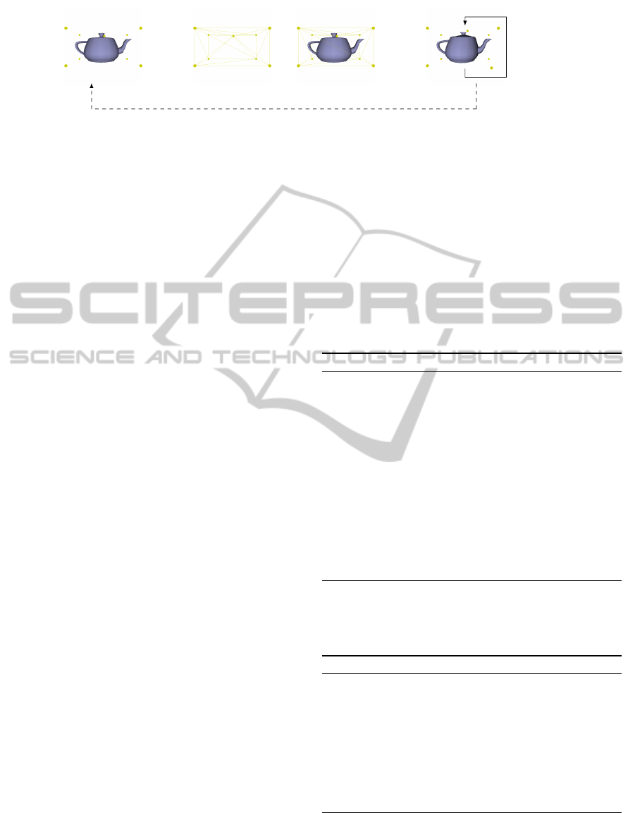
Figure 2 shows a 2D example of the supporting

structure that is obtained by our algorithm.

GRAPP2013-InternationalConferenceonComputerGraphicsTheoryandApplications

112

Initial situation

Nested partitions

Figure 2: Convex partitions in the 2D case (framed in red).

4 COMPUTATION OF THE GBC

The next step is to compute the GBC that relate the

model with the control points.

Our system has to deal with multiple convexes

which are arranged in two partitions. Each of these

convexes contains parts of the mesh to be deformed

and each partition contains the whole mesh. This

means that the GBC system used must ensure the con-

tinuity between all the convexes in the same partition

(the GBC on a face must coincide for the left and right

convexes of this face).

The coordinates of a vertex p of the polygonal

mesh are computed in three steps:

1. Compute the set Convexes of p (Θ

): for each par-

tition P

, ﬁnd the convex θ

that contains p:

= {θ

: p ∈ θ

∧ θ

∈ P

, j ∈ {0, 1}} (4)

2. For each convex θ

of Θ

, compute the set of co-

ordinates of p w.r.t θ

(α

(p),α

(p),...,α

m−1

(p)), (5)

where M = |Q|.

3. Compute the ﬁnal coordinates as a convex combi-

nation of the coordinates for each θ

in Θ

(p) =

∑

j=0

(p)

(p) =

∑

j=0

(p)

m−1

(p) =

∑

j=0

m−1

(p), (6)

where

∑

j=0

= 1 and ω

|Θ

The coordinates in Step 2 are calculated using one

of the existing systems of GBC that coincide on the

boundaries of the convexes. In our implementation,

we have chosen the MVC.

See Figure 3 for an example of the inﬂuence of the

control points over the mesh of the model.

Figure 3: Inﬂuence regions of two different control points.

Red colors correspond to higher values of the coordinate.

The complete connectivity is also shown for a better under-

standing.

4.1 Properties Discussion

Constant precision:

∑

(p) = 1 ∀p

Proof:

∑

(p) =

∑

j=0

∑

(p)

(7)

MVC have this property which, together with

Equation 6, implies:

∑

(p) =

∑

j=0

= 1 (8)

Linear precision: p =

∑

(p) ∀p

Proof:

∑

(p) =

∑

j=0

∑

(p)

(9)

MVC have this property, which, together with

Equation 8, implies:

∑

(p) =

∑

j=0

p = p

∑

j=0

= p (10)

Convex combination: α

(p) ≥ 0 ∀i, ∀p

Proof:

(p) =

∑

j=0

(p) (11)

Knowing that MVC have this property over con-

vex polytopes, the property is concluded being:

j ∈ {0,1} (12)

Smoothness

The smoothness of the coordinates of our system is

inherited by the existing coordinates system used in

Step 2 (see Section 4). In our case, the chosen system

is the MVC. For this reason, the ﬁnal coordinates of

our method present C

∞

continuity inside the convexes

(they are smooth) and C

continuity on their bound-

aries.

Cage-freeSpatialDeformations

113

5 RESULTS AND DISCUSSION

In this section we present some of the examples over

which we have tested our deformation system. The

computer used in these tests is equipped with an Intel

Core2Duo E8400 3.00GHz CPU with 4GB of RAM

and running Ubuntu 11.10 as O.S.

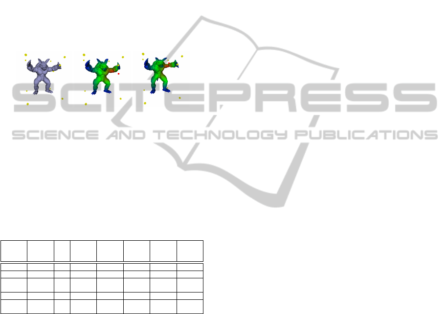
Figure 4 shows a deformation sequence using the

Armadillo model mesh. For this example we have set-

up 8 surrounding control points and 2 more positioned

near the hand and the elbow of the Armadillo. Notice

that the control point located near the hand allows to

keep it in a more constant position while the control

point in the elbow is displaced.

Figure 4: Local deformation on the Armadillo. The ﬁrst

image is the initial position. The next two images show the

effect of displacing the control vertex close to the elbow.

We have also evaluated the time needed to com-

pute the connectivity between the control points and

the GBC using these structures. The obtained data is

shown in Table 1.

Table 1: Time needed to automatically compute the con-

nectivity between the control points and the coordinates for

different well-known models.

Model

points

|Q|

Interior

Con

vexes

Connec

tivity

(ms)

GBC

(ms)

Total

(ms)

Teapot 529 13 5 25 0.39 4.73 5.12

Bunny 35947 13 5 25 0.39 223.58 223.97

Arma

dillo

172974 14 6 28 0.43 1102.61 1103.04

Dragon 437645 14 6 28 0.40 2533.25 2533.65

Happy

Buda

543652 14 6 28 0.40 3363.91 3364.31

Analyzing the results, we observe that most of the

cost of our algorithm lies in the coordinates compu-

tation. Notice that each partition contains the entire

mesh of the model. In our case, the model has to be

processed twice so the computation of the coordinates

will be at least twice slower than in the classical cage-

based methods.

6 CONCLUSIONS

We have presented a new method for interactive mesh

deformation which does not need any explicit deﬁni-

tion of the structure between the control points. The

user is only responsible of the deﬁnition of these con-

trol points, being allowed to locate them wherever he

wants. Our method will automatically compute a con-

nectivity between them to support the computation of

the GBC used to deform the mesh. We have also pre-

sented all algorithms needed to reach our goal.

Our future work will be centered on the study of

new algorithms that improve the creation of the con-

nectivity between control points. Another main line

of work is the parallelization of the algorithms to de-

crease the time used in the computation of the GBC.

ACKNOWLEDGEMENTS

This project has been funded by the Universitat

Politcnica de Catalunya (UPC) and by the project

TIN2010-20590-C02-01 of the Spanish Government.

We wish to thank the reviewers for their helpful

suggestions which have been taken into acconut.

REFERENCES

Floater, M. S. (2003). Mean value coordinates. Computer

Aided Geometric Design, 20(1):19–27.

Floater, M. S., Hormann, K., and Ks, G. (2006). A gen-

eral construction of barycentric coordinates over con-

vex polygons. In Advances in Computational Mathe-

matics, pages 311–331.

Floater, M. S., K

os, G., and Reimers, M. (2005). Mean

value coordinates in 3d. Comput. Aided Geom. Des.,

22(7):623–631.

Joshi, P., Meyer, M., DeRose, T., Green, B., and Sanocki,

T. (2007). Harmonic coordinates for character articu-

lation. ACM Trans. Graph., 26(3):71.

Ju, T., Schaefer, S., and Warren, J. (2005). Mean value

coordinates for closed triangular meshes. ACM Trans.

Graph., 24(3):561–566.

Li, Z., Levin, D., Deng, Z., Liu, D., and Luo, X. (2010).

Cage-free local deformations using green coordinates.

Vis. Comput., 26(6-8):1027–1036.

Lipman, Y., Kopf, J., Cohen-Or, D., and Levin, D.

(2007). Gpu-assisted positive mean value coordi-

nates for mesh deformations. In Proceedings of the

ﬁfth Eurographics symposium on Geometry process-

ing, SGP ’07, pages 117–123, Aire-la-Ville, Switzer-

land, Switzerland. Eurographics Association.

Lipman, Y., Levin, D., and Cohen-Or, D. (2008). Green

coordinates. ACM Trans. Graph., 27(3):1–10.

Mbius, A. F. (1827). Der Barycentrische Calcul. Johann

Ambrosius Barth, Leipzig.

Meyer, M., Barr, A., Lee, H., and Desbrun, M. (2002).

Generalized barycentric coordinates on irregular poly-

gons. J. Graph. Tools, 7(1):13–22.

Wachspress, E. L. (1975). A Rational Finite Element Basis.

Academic Press, New York.

GRAPP2013-InternationalConferenceonComputerGraphicsTheoryandApplications

114