
A Two-step Empirical-analytical Optimization Scheme
A Simulation Metamodeling Approach
Wa-Muzemba and Anselm Tshibangu
University of Maryland Baltimore County, Department of Mechanical Engineering,
1000 Hilltop Circle, Baltimore, Maryland 21250, U.S.A.
Keywords: Optimization, Robust Design, Simulation Meta-modeling.
Abstract: This paper presents a two-step optimization scheme developed to find the optimal operational settings of
operational systems seeking to optimize their operations using multiple performance measures. The study
focuses on two conflicting performance measures, the Throughput Rate (TR) and the Mean Flow Time
(MFT). First an empirical approach is used to uncover the near optimal values of the performance measures
using an experimental design procedure. Second, an analytical procedure is deployed to find the exact
optima using values the near optima found in the first step as target. The analytical procedure uses a non-
linear regression meta-model derived from simulation outputs and compromises the two conflicting targets
while minimizing the loss incurred to the overall system. This loss is expressed in the form of a multivariate
version of the Taguchi quadratic loss function. Although the framework as presented in this paper is derived
by analyzing a manufacturing system through discrete-event simulation, the procedure however, can
successfully be applied to any processing system in various industries including food production, financial
institutions, warehouse industry, and healthcare.
1 INTRODUCTION
The choice of performance measures in a processing
system depends highly on management policy and
decision-making. Multiple objective measures are
needed to describe the dynamic nature of a
production system. A single performance measure is
not enough to capture and characterize the overall
performance of a system. Also, optimizing a system
with respect to one single objective only may lead to
sacrificing other objective(s) of interest. For
example the objective of minimizing in-process
inventory might be in conflict with that of
maximizing a production rate. Literature on the
design and operation of flexible manufacturing
systems has shown that most of the past research
studies have used only a single performance measure
in their objective functions (Blogun et al., 1999).
From this point of view, the multi-objectives
approach has recently been of interest in a wide
range of design and control problems for
manufacturing systems, such as machine selection,
choice of the manufacturing or processing system
configuration architecture, control of automated
storage and retrieval systems, and overall scheduling
scheme.
The selection of the most appropriate setting of
input factors in order to attain the required process
objective/target (mean) is of major interest in a
variety of production environments. The problem is
referred to as the “optimal setting parameters”
because it is concerned with selecting the best
setting of parameters for an optimal operation of the
system. It worth it to mention that the generic term
of system is used in this study to designate a
process-oriented infrastructure including a
warehouse, a manufacturing system, or a operating
theater in a hospital. Selecting the optimal setting is
critically important since it affects not only
performance measures, operations and/or production
costs but also the loss incurred to the system in the
event of a performance deviation from the company-
identified target values. On the other hand, these
operational targets need to be frequently reviewed as
a result of the unpredictable variations in the shop
floor conditions and the fluctuating nature of the
market place.
Clearly, there is a true need and a real
opportunity to apply a combined scheduling
methodology to dynamic and stochastic scheduling
problems with the objective of reducing the overall
558
Tshibangu W. and Tshibangu A..
A Two-step Empirical-analytical Optimization Scheme - A Simulation Metamodeling Approach.
DOI: 10.5220/0004489105580565
In Proceedings of the 10th International Conference on Informatics in Control, Automation and Robotics (ICINCO-2013), pages 558-565
ISBN: 978-989-8565-71-6
Copyright
c
2013 SCITEPRESS (Science and Technology Publications, Lda.)

production cost.
This paper analyzes a hypothetical flexible
manufacturing system using simulation and proposes
a unique and robust scheme in designing, modeling
and optimizing systems in a very effective way. The
reader is referred to other author’s publications
(Bardhan and Tshibangu, 2003), (Tshibangu, 2005),
(Tshibangu, 2006) for a detailed description of the
hypothetical manufacturing system considered in
this study. The system is modeled with a total
number of 9 workstations including a receiving and
a shipping stations. These 9 stations process are
served by a fleet of AGVs while processing fifteen
part types, each with a different processing time.
The optimization procedure as developed in this
paper is carried out at two levels. First an empirical
approach is used to uncover near-to-optimal values
of the individual performance criteria of interest.
These values are subsequently used as targets in the
second and more analytical level of the optimization
procedure during which a multi-criteria optimization
technique eventually uncovers the true optimal
setting of the system parameters. Specifically, the
analytical optimization is applied to a regression
model equation (meta-model) derived from
simulation output results. The approach used in this
study takes advantage of a robust experimental
design methodology to render the system immune to
noise. The purpose is to present a pragmatic
approach that may enhance the overall performance
of process-oriented systems including manufacturing
systems, warehouse, airport traffic and hospitals.
2 RESEARCH METHODOLOGY
The various phases of the robust design
methodology as applied in this paper is the same as
proposed in the literature (Montgomery 2012),
(Taguchi, 1987) except that in this study, after
completing the simulation experiments and
collecting alll pertinent data the following additional
steps are taken in order to accommodate the
subsequent optimization procedures as proposed in
this research:
(1) Calculate the mean and the variance with respect
to noise factors
2
wrtnf(i)
for each treatment i (row
of the inner array) and for each performance
measure of interest; this variance measures the
variation in the performance criterion when there
is a change in noise factors.
(2) Compute and use log
2
wrtnf(i)
of each
performance measure to improve statistical
properties of analysis.
(3) Apply the normal probability plotting technique
to the calculated mean and the log
2
wrtnf
of each
control factor setting to determine the
significance of the main factors and their
interaction effects on each performance measure
of interest.
(4) Develop and implement the four-step
optimization procedure to predict the factors and
their associated settings that will simultaneously
minimize
2
wrtnf
and optimize the mean of the
performance measures. Adjust and fine-tune the
settings to the most appropriate economical
levels.
(5) Perfom a second analytical optimization
procedure using a Bi-variate Quadratic Loss
Funtion (BQLF) inspired from Taguchi
Methodology
(6) Run confirmatory simulation experiments.
(7) Make the conclusions on the multi-criteria
optimization procedure.
2.1 The Robust Design Formulation
Implementing the robust design formulation requires
the following steps:
Define the response or dependent variables
(performance measures of interest), the
independent variables (including the controllable
factors and the uncontrollable factors or source
of noise ).
Plan the experiment by specifying how the
control parameter settings will be varied and how
the effect of noise will be measured.
Carry out the experiment and use the results to
predict improved control parameter settings (e.g.,
by using the optimization procedure developed in
this study).
Run a confirmation experiment to check the
validity of the prediction.
This study takes advantage of a robust design
configuration inspired by the Taguchi robust design
methodology. However, because of the high amount
of criticism against Taguchi’s experimental design
tools such as orthogonal arrays, linear graphs, and
signal-to-noise ratios, this study avoids the use of
Taguchi’s statistical methods but rather uses an
empirical technique developed by the author.
The paper develops and proposes an optimization
scheme by studying an AGV-served FMS and
evaluating its overall performance using the mean
flow time (MFT) and the throughput rate (TR). The
study considers as controllable variables 5 design
parameters, designated by X
i
(i=1…5), namely: i) the
number of AGVs (X
1
), ii) the speed of AGV (X
2
), iii)
ATwo-stepEmpirical-analyticalOptimizationScheme-ASimulationMetamodelingApproach
559

the queue discipline (X
3
), iv) the AGV dispatching
rule (X
4
), v) and the buffer size (X
5
). These variables
have a direct impact on the performance of machines
and material handling (AGVs) as they are
considered in most literature not only as the most
expensive (some even as the most sensitive)
components of the overall system and also as
potential sources of operational disturbances. The
natural values assigned to these design variables are
displayed in Table 1. In this study, the controllable
parameters X
1
through X
5
to set and tested at two
setting levels (min and max).
The principal sources of noise tested in this study
(and also considered as the most commonly
investigated and documented in the reported
literature (Montgomery, 2013) are: i) the arrival rate
between parts (or orders), (X
6
), the mean time
between failures of the machines (X
7
) and the
associated mean time to repair (X
8
). These factors
are also tested at two levels in combination with
each control factor (X
1
through X
5
) at each setting
level.
Table 1: Natural values and setting of control factors.
Designation Control Factor
Low
Level (-1)
High
Level (+1)
X
1
Number of AGVs 2 9
X
2
Speed of AGV 100 200
X
3
Queue Discipline FIFO SPT
X
4
AGV Dispatching Rule FCFS SDT
X
5
Buffer Size 8 40
Table 2 depicts settings and natural values for noise
factors as assigned and simulated in the experiments.
For both controllable and noise factors, the coded
levels are (-1) and (+1) for the low and high level,
respectively.
2.2 Planning the Experiment
Planning the experiment is a two-part step that
involves deciding on how to vary the parameter
settings and how to measure the effect of noise
(Kacker and Shoemaker, 1986). Using a full
factorial experimental design with the 5 controllable
factors X
1
, X
2
, X
3
, X
4
, and X
5
set at two levels in
combination with three noise factors X
6
, X
7
, and X
8
,
varied at two settings would require 2
5
x 2
3
= 256
simulation runs.
Two-level, full factorial or fractional factorial
designs are the most common structures used in
constructing experimental design plans for system
design variables. Montgomery (2013) recommends
appropriate fractional factorial designs of resolution
IV or V in the design of robust manufacturing
systems. In this study a two-level fractional factorial
design of resolution V, denoted 2
v
5-1
has been used.
This design requires only 16 runs. Across the full set
of noise factors, the implemented robust design
leads to a total of 16 x 8 = 128 simulation runs
(instead of 256 as required by a full factorial
design). The study also decides to use a robust
design of resolution V in order to allow an
estimation of both main factors and two-way
interactions effects, as they are necessary and very
crucial for the first step of the proposed optimization
scheme, and referred to as the empirical step.
A standard statistical experimental design, also
known as a data collection plan is normally
advocated and recommended when conducting
simulation experiments. The data collection plan
used in this study was inspired from Genichi
Taguchi’s strategy for improving product and
process quality in manufacturing (Taguchi, 1986). It
has been first used and proposed by Wild and
Pignatiello (Wild et al., 1991). Their proposed
design strategy includes simultaneous changing of
input parameter values. Therefore, the uncertainty
(noise) associated with not knowing the effect of
shifts in actual parameter values such as shifts in
mean inter-arrival times, mean service times, or the
effect of not knowing the accuracy of the estimates
of the input parameter values, is introduced into the
experimental design itself. Tshibangu, 2003, 2005
provides detailed information about this specific
data collection plan. This plan has been also used in
this study to run the simulation experiments and
effectively collect the statistics thereof.
Table 2: Natural values and setting of noise factors.
Designation Noise Factor Low Level (-1) High Level (+1)
X
6
Inter-arrival EXPO(15) EXPO(5)
X
7
MTBF EXPO(300) EXPO(800)
X
8
MTTR EXPO(50) EXPO(90)
3 EMPIRICAL OPTIMIZATION
Because flexible manufacturing systems and any
other process-oriented systems are subject to various
uncontrollable factors that may adversely affect their
performance, a robust design of such systems is
crucial and unavoidable. The author has developed a
four-step optimization procedure to be used
simultaneously with the robust design as first step of
the optimization scheme as proposed in this study:
Let
i
y
represent the average performance
measure across all the set of noise factors
ICINCO2013-10thInternationalConferenceonInformaticsinControl,AutomationandRobotics
560

combination, averaged across all the simulation
replications for each treatment combination (or
design configuration) i. Let log
2
wrtnf(i)
be the
associated logarithm of the variance with respect to
noise for that particular treatment i. Kacker and
Shoemaker, 1986 recommend to use the logarithm
of the variance in order to improve statistical
properties of the analysis, and to employ the
“effects” values and/or graphs in association with
normal probability plots and or ANOVA procedures
to identify and partition the following three
categories of control factor vectors:
Assuming that we have partitioned three
categories of control vectors as non-empty sets X
v
T
containing the factors that have a significant effect
on the variances, X
m
T
containing factors significant
on the means (and their interactions), and X
0
T
as the
set of the factors that affect neither the mean nor the
variance, respectively, then a four-step empirical
optimization procedure may be implemented as
follows:
1. Step 1
Identify the vector X
v
T
and adjust the controllable
factors members of this set to their values that
minimize
2
wrtnf
.
of the performance measure y.
2. Step 2
Identify vector (X
m
T
)
1
of factors having a significant
effect on the mean
y
and set the controllable factors
members of this set to their level values that
optimize the mean
y
of the objective performance
y. Also, identify (X
m
T
)
2
vector of factors having a
significant effect on mean
y
and on the variance
2
wrtnf
simultaneously and set the factor members of
this set to their level values that optimize the mean
y
if this setting does not act in opposition with the
minimization of the variance. Otherwise, find a
compromise between minimizing the variance and
optimizing the mean as suggested in Step 4 where
the final setting is to be decided.
3. Step 3
Identify the vector X
0
T
and set the control factors
members of this set to the values of their interaction
with members of vector X
v
T
that minimize the
variance or log
2
wrtnf
or the values of their
interaction with members of X
m
T
that optimize the
mean
y
. Otherwise, set the factors at their
economical settings.
4. Step 4
Conduct a small follow-up experiment to find trade-
off between members of (X
m
T
)
2
B
containing factors
with effects on variance and mean acting in
opposition and or the overall economical settings. A
suggestion from this study is that in finding the
overall economical setting, the step involves only
those factors that have the greatest effect on either
the variance
2
wrtnf
or the mean
y
.
Using the above-developed procedure with
related plots and tables, and applying it to the data as
derived from the experiments for the two
performance measures, i.e., Mean Flow Time (MFT)
and Throughput Rate (TR) performance measures,
the following coded results are obtained: MFT =
0.3666 units time/part and TR = 3000 parts/month
(100 parts/day). These values will be considered as
the optimal target values to be achieved in the
second level of the optimization procedure (multi-
criteria optimization).
3.1 Simulation Meta-modeling
Tshibangu (2005) redefines the purpose of meta-
modeling as the method by which to measure the
sensitivity of the simulation response to various
factors that may be either decision (controllable)
variables or environmental (non-controllable)
variables (Kleijnen, 1977).
After completing the robust design process, the
128 simulation experiments were carried out as
initially recommended in the experiment plan and
the main statistics describing the system were
collected following the proposed data collection
plan. These values were subsequently fed into a non-
linear regression meta-model to derive the estimate-
equations
ˆ
TR
y
and
ˆ
M
TF
y
for the throughput rate
(TR) and the mean flow time (MFT), respectively.
Meta-models are usually constructed by running a
special RSM (Response Surface Methodology)
experiment and fitting a regression equation that
relates the responses to the independent variables or
factors.
3.2 Determination of Variances, Main
and Interaction Effects
A well-planned experiment makes simple the
analysis subsequently needed to predict the
improved (optimal) parameter settings. In this study,
for each of the simulated design configurations i,
eight measurements (over the set of noise factor
combinations) were taken for each performance
measure of interest and averaged across the
replications to obtain
i
y
for each i
th
row of the inner
array. Sixteen design configurations and five center-
points (for a total of 21) designs were simulated over
a set of eight noise factor combinations, leading to
ATwo-stepEmpirical-analyticalOptimizationScheme-ASimulationMetamodelingApproach
561
21x8 =128 runs. The results of these various
simulation experiments, too large to be displayed in
this paper, but available upon request, were
subsequently averaged up across the three
replications.
This research intends to minimize the variances
of the performance measures with respect to the
noise factors for each run. The reported variances
across the text, denoted [
2
(wrtnf)
] is calculated as
follows:
2
(wrtnf)
i
2
1
1
, 1, 2,... ,
1
f
ij
i
j
yy j f
f
(1)
where y
ij
is the observed value of a given
performance measure for a particular design
configuration i and a noise factor configuration j;
y
is the average value of a given performance
criterion considering that particular design
configuration i. In this study, f = 8 (eight noise
combinations).
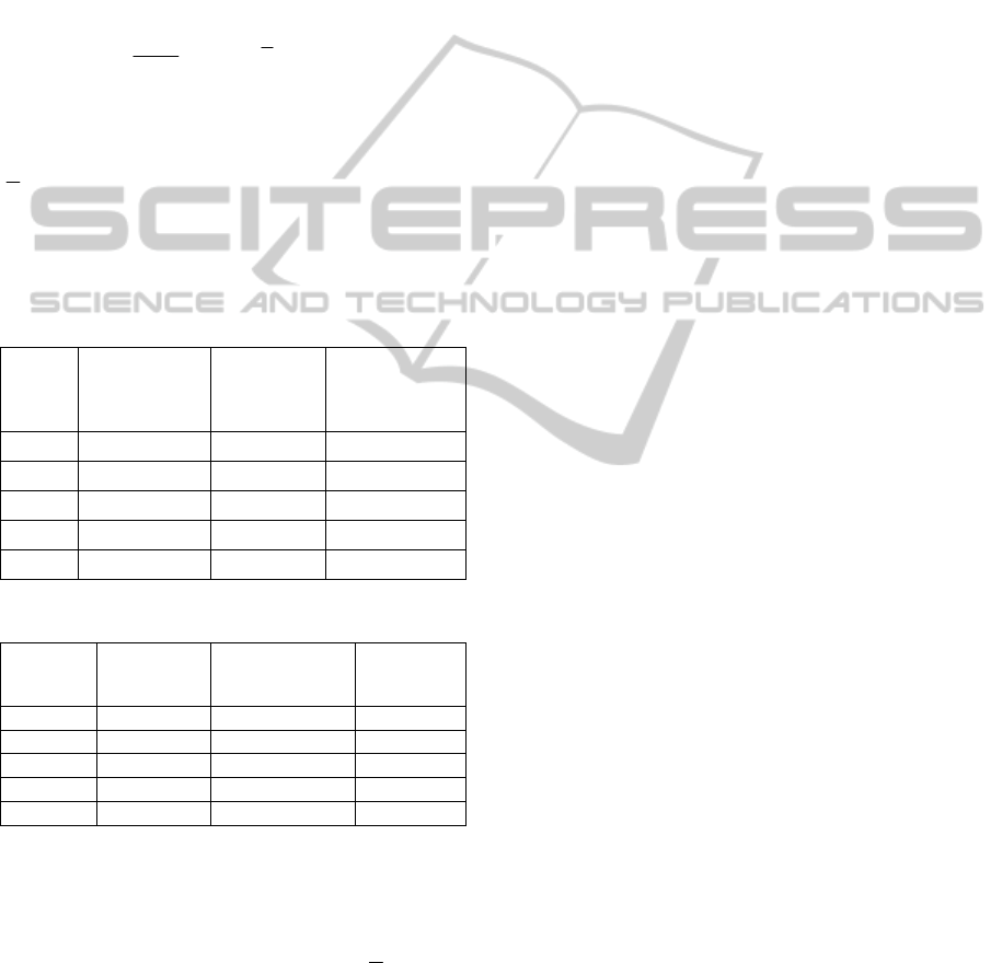
Table 3: Effects of Control Factors MFT Variance.
Control
Factors
Effect on MFT
log
2
wrtnf
at Level (+1)
Effect on
MFT log
2
wrtnf
at Level (-1)
Absolute Value
Difference
between High
and Low levels
X
1
1.6159 1.657502 0.04155
X
2
1.6081 1.558286 0.04982
X
3
1.4921 1.781325
0.28920
X
4
1.6338 1.639566 0.00568
X
5
1.6032 1.670230 0.06701
Table 4: Effects of Control Factors on MFT Mean.
Control
Factors
Effect on MFT
Average
Level (+1)
Effect on MFT
Average
at Level
(-1)
Absolute
Value
Difference
X
1
8.238767 25.97234
17.73358
X
2
12.62954 20.89605 8.26650
X
3
13.86047 20.35063 6.49016
X
4
16.97108 17.24002 0.26893
X
5
17.61093 16.60017 1.01076
The objective is to make the variances of the
responses (performance measures) as small as
possible while the means are brought to their
optimum settings, which would consists of a
minimum for the MFT and a maximum for the TR.
The study then computes the values of
i
y
and log
2
(wrtnf)i
at each design configuration. Subsequently,
the effects of each control factor on the overall mean
and the variance (or log
2
wrtnf
) are calculated by
using the normal probability data plotting technique
(Box et al., 1978). Tables 3 and 4 display the effects
on the MFT variance and mean, respectively.
As it can be seen, these effects on the mean and
the variance are also partitioned into high level and
low level effects. The same procedure is applied to
the throughput rate TR and the results, not displayed
in this paper, are available upon request. The process
is conducted for all the control factors. Then each
controllable factor is tested at two levels, the
magnitude of its effect on variability is measured by
the difference between the average values of log
2
wrtnf
at those settings. The computed effects at high
and low levels will be used in identifying those
controllable factor levels (settings) that have the
largest effect on log
2
wrtnf
. The same procedure is
also applied to the mean values to determine the
effects of the control parameters. Note that a visual
summary of the magnitude of each control factor’s
effect can also be used for analysis of various
effects. From analysis of the results in Table 3 for
example, it can be seen on one hand for instance (in
bold) that the parameter X
3
(queue discipline) has
the most significant effect on the MFT variability.
These results agree with previous findings (Egbelu
and Tanchoco 1984); (Sabuncuoglu, 1989);
(Bardhan and Tshibangu 2003). On the other hand,
the effect at high level is compared to the effect at
low level, and the better setting of each control
parameter is the one that gives the smaller average
value of log
2
wrtnf
. Table 4 results indicate that
factor X
1
(the number of AGVs), when set at its high
level, has the most significant effect on the mean
value of the MFT (see results in bold). Once
identified, these factors will be set at the settings
(levels) that minimize log
2
wrtnf
., i.e., X
1
and X
3
at
high settings. Proceeding the same way for the TR
similar results are obtained and the settings
implemented.
Now that the first empirical optimization step has
revealed the near optimal settings of the system, it
becomes appropriate to move to the second step of
the optimization procedure, referred to in this study
as the analytical phase of the proposed optimization
scheme. For one to perform the analytical
optimization step, a mathematical model of the
system is required. This paper proposes to feed the
simulation results into a non-linear regression meta-
model to derive the mathematical model. Applying
the meta-modeling technique to the flexible
manufacturing system under study in this research
yield the following equations for the estimates of
two performance measures of interest,
ˆ
TR
y
and
ˆ
M
TF
y
.
ICINCO2013-10thInternationalConferenceonInformaticsinControl,AutomationandRobotics
562

12
22
3512
222
34512
13 23 34
ˆ
90.7617 20.6726 2.5357
2.6977 0.5617 4.712 9.042
8.732 4.712 7.923 7.458
3.5513 0.5315 0.3304
TR
yxx
x
xxx
x
xxxx
xx xx xx
(2)
12
345
222
123
22
4512
13 14 15
23 24 35
45
ˆ
4.6503 8.8668 4.4760
3.2451 0.1345 0.5054
14.1731 1.5309 1.3399
0.4519 1.4569 5.3816
0.7952 0.0335 0.504
0.1457 0.3251 0.4863
0.7655
MFT
yxx
xxx
xxx
xxxx
x
xxxxx
x
xxxxx
xx
(3)
where
54321
,,,, xxxxx are the coded units for the
operating variables X
1
, X
2
, X
3
, X
4
, and X
5
,
respectively.
4 ANALYTICAL APPROACH
The Taguchi’s loss function discussed in the
literature (Montgomery, 2013) for a single objective
criterion can be extended to the case of multiple
quality characteristics or objective performances,
and then referred to as a “multivariate quality loss
function”. The author (Tshibangu, 2006) shows how
the traditional and simple QLF can be extended to a
multivariate QLF.
Let y
j
, and T
j
be the performance measures of
interest (j =1 to Q, where Q is the total number of
performance measures), and the target for objective
performance
j
y
, respectively, and be denoted by y =
(y
1
, y
2
,…, y
Q
)
T
and T = (T
1
, T
2
,…, T
Q
)
T
under the
assumption that L(y) is a twice-differentiable
function in the neighborhood of T.
Assuming that each objective performance has a
mean
(x)
i
and a variance
(x)
i
2
, then, after some
mathematical developments and manipulations
(Tshibangu, 2005), (Ribeiro and Elsayed, 1995) the
expected value of the quadratic loss function for a
bivariate QLF can be derived and written as follows:
2
2
2
12
1
12 1 1 2 2
(, )
iii i
i
ELy y T
yTyT
(4)
The first term of the second hand side of Eqn. (4) is
known as a weighted sum of mean squares, while
the second term is called the gradient term. It is
important to note that three aspects are of interest in
formulating robust design systems:
(i) deviation from targets; (ii) robustness to
noise; (iii) robustness to process parameters
fluctuations. A weighted sum of mean squares is
appropriate to capture (i) and (ii), while gradient
information is necessary to capture (iii). This
research is particularly interested in deviation from
target and robustness to noise. Therefore, only the
first term of Equation (9) is needed.
The next step consists of applying the derived
QLF to the FMS meta-models Eqns. (2) and (3)
obtained from simulation outputs. In order to
determine the optimal input parameters, an objective
function is developed from Eqn. (4), following a
framework adopted by Ribeiro and Elsayed (1995).
Because of the robust design configuration
adopted during the experiments, it can be assumed
that the variability of the system due to fluctuations
of the operating parameters is negligible, then, for a
given treatment, the loss incurred to a system as the
result of a departure of the system performance
j
y
from the target T
j
can be estimated as:
2
1
ˆˆ
()
Q
j
jj yj
i
i
Li w y T
(5)
where
()
L
i
is the loss at treatment i;
j
w
is a weight
to take into account in order to consider the relative
importance of a individual performance measure
j
y
(j=1,2,…Q),
ˆ
,
jyj
y
are respectively the
predicted (estimate) mean and standard deviation of
the performance measures of interest
j
y
, and
j
T
is
the target for the system performance measure
j
y
.
L(i) is the objective function to be minimized. In this
particular form, the objective function has two
terms. The first term of the objective
function,
2
ˆ
jj
y
T , accounts for deviations from
target values. The second term,
2
ˆ
yj
accounts for
the source of variability due to non-controllable
factors (noise).
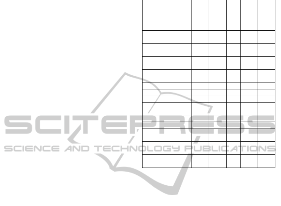
5 RESULTS
For the twenty-one treatment combinations
simulated in this study, the resulting normalized
values are displayed in Table 5 showing the values
ATwo-stepEmpirical-analyticalOptimizationScheme-ASimulationMetamodelingApproach
563
of
j
y
and
2
log
yj
at each design configuration
for each of the two primary performance criteria of
interest in this study. Note that only the throughput
rate (TR) seeks a maximization. The mean flow time
(MFT) and the variances of both TR and MFT need
be minimized. Therefore, the normalization
procedure of these values will consist of maximizing
the inverse. Further analysis of output results
indicates that design configurations labeled #3, 7,
16, 20, and 21 are the most cost effective as they
yield the least cost. This finding suggests that
operating the studied system under any of these
design settings would be far more economically
attractive than operating the same system under
other design settings even when they are also
identified as the most robust designs. For example,
the difference between the most cost-effective
design (configuration design #3) and the most
expensive one (design #13) represents
approximately 56 monetary units in normalized
values. This may represent a significant amount of
money if the value of the monetary loss coefficient
factor is important. Using for example $10.00 value
for the loss coefficient will lead to a difference of
$123.00 in expected losses between design # 3 and
design # 13 representing
38
(1 ) *100 76%
161
of
savings when operating under design # 3 setting
parameters. Design #13 has been used for the
comparison because it is among the strongest design
candidates in terms of robustness of the system (i.e.,
insensitivity to noise factors). This example shows
that significant savings (e.g. 76%) can be generated
when switching ample from design #13 to design #3.
6 CONCLUSIONS
This stud first uses an empirical optimization
procedure to avoid the controversial Taguchi
statistical tools. Then a metamodel is derived from
the simulation outputs. The study also derives a
multivariate quadratic loss function (QLF) from the
traditional Taguchi loss function in order to capture
the loss incurred to the overall system when
attempting to optimize a set of two objective
performances (throughput rate TR and mean flow
time MFT). Hence, the QLF is referred in this study
to as a bivariate quadratic loss function (BQLF).
Table 5: Normalized input data and predicted loss.
Design
Configuration
TR
TR log
(Var)
MFT
MFT
log
(Var)
Pred.
Loss
e.g. K=
$10.00
Norm Norm Norm Norm L(i)
Loss in
$
Design 1 0.056 -0.001 0.034 0.008 21.158 212
Design 2 0.020 0.845 0.009 0.032 59.481 594
Design 3 0.068 -0.007 0.079 0.075 3.792 38
Design 4 0.018 -0.212 0.012 0.007 57.632 576
Design 5 0.056 -0.002 0.036 0.010 18.947 189
Design 6 0.032 -0.097 0.030 0.013 54.482 545
Design 7 0.068 -0.007 0.079 0.075 3.792 38
Design 8 0.034 -0.795 0.021 0.046 53.631 536
Design 9 0.035 -0.299 0.020 0.051 52.277 522
Design 10 0.065 -0.004 0.095 0.114 6.142 61
Design 11 0.019 0.477 0.011 0.010 58.599 586
Design 12 0.033 1.429 0.023 0.026 54.035 540
Design 13 0.057 -0.002 0.087 0.088 16.118 161
Design 14 0.049 -0.001 0.026 0.006 31.707 317
Design 15 0.066 -0.005 0.081 0.076 4.958 50
Des 16 0.068 -0.007 0.079 0.075 3.792 38
Design 17 0.058 -0.002 0.087 0.088 15.599 156
Design 18 0.049 -0.001 0.026 0.006 31.137 311
Design 19 0.019 -0.295 0.009 0.043 59.900 599
Design 20 0.068 -0.007 0.079 0.075 3.792 38
Design 21 0.068 -0.007 0.079 0.075 3.792 38
Next (second level of the optimization scheme), the
BQLF is analytically applied to the metamodel
derived from the simulation outputs to fine-tune the
ptimization process em with respect to the two
objective performances. From the results obtained in
step 1 of the optimization scheme as developed in
this paper, optimum/target values of 100 parts/day
and 0.3666 units time/part (in coded data) have been
fixed for the TR, and MFT, respectively.This two-
level optimization procedure lead to a solution that
yield a minimum cost to be incurred to the overall
system as a penalty for missing the objective targets.
The values of 98 parts/day (-2% from target) and
0.3459 units time/part (+5.6% from target) are
obtained as optima, for TR and MFT, respectively.
These maximum outputs will be otained under a
overal system configuration that is considered to be
the most robust and economical, leading to the
following settings in natural values: Number of
AGVs (X
1
): 6; Speed of AGV (X
2
): 150 feet/min;
Queue discipline (machine rule) (X
3
): SPT; AGV
dispatching rule (X
4
): STD; Buffer size: (X
5
): 4.
Although, conceptually validated on a flexible
manufacturing system, the above-developed and
proposed optimization scheme can be easily
extended to other process-oriented industries
including banks, warehouse, ticketing lines at
airports, restaurants, healthcare facilities,
phamaceutical industries, and others.
ICINCO2013-10thInternationalConferenceonInformaticsinControl,AutomationandRobotics
564

REFERENCES
Bardhan, T. K, and Tshibangu W. M. A. 2003. Analysis of
an FMS with Considerations of Machine Reliability,
Proceedings of 8
th
Annual IJIE Engineering Theory,
Applications and Practice, Las Vegas, Nevada, US
Kacker, R. N., Shoemaker, A. C., Robust Design, 1986. A
Cost Effective Method for Improving Manufacturing
Processes., AT&T Technical Journal, Volume 65, 51-
84.
Kleijnen, J. P. C., Design and Analysis of Simulations,
1977. Practical Statistical Techniques, SIMULATION,
Volume 28, no.3, 81-90.
Montgomery, D. C., 2013, Design and Analysis of
Experiments, (Eighth Edition, New York: John Wiley
& Sons Inc.
Ribeiro, J. L., and Elsayed, E. A., 1995. A Case Study on
Process Optimization Using the Gradient Loss
Function, International Journal of Production
Research, Volume 33, no. 12, .
Taguchi, G., 1986. Introduction to Quality Engineering-
Designing Quality Into Products and Processes, Asian
Productivity Organization, Tokyo.
Tshibangu W. M. A., 2005. A Framework for Designing a
Robust Material Handling Using Simulation and
Experimental Design, Proceedings of the 10
th
IJIE
Conference Florida.
Tshibangu, W. M. 2006, Robust Design of an FMS: S. M.
Proceedings of the GCMM, COPEC, Council of
Researches in Education and Sciences November19-
22, Santos, Brazil.
Wild, R. H., and Pignatiello, J. J., Jr., 1991.An
Experimental Design Strategy for Designing Robust
Systems Using Discrete-Event Simulation,
SIMULATION, Volume 57, no.6, 358-368.
ATwo-stepEmpirical-analyticalOptimizationScheme-ASimulationMetamodelingApproach
565
