
User-guided Modulation of Rendering Techniques for Detail Inspection
Ankit Sharma and Subodh Kumar
Department of Computer Sc. and Engg., Indian Institute of Technology Delhi, New Delhi, India
Keywords:
Feature based shading, Detail enhancement.
Abstract:
Understanding intricate details of carved models, for example ones prevalent in cultural heritage applications,
is often difficult from renderings using traditional illumination models. A number of illustrative rendering
techniques are known, but each works well only for some models. We present a rendering system that com-
bines these techniques in an attempt to make the visualization more comprehensible given any context. In
particular, our system learns user’s visual preferences using exemplars from a domain and applies an appropri-
ate combination of the basis techniques to new meshes from that domain. Given a polygonal mesh, the system
applies different rendering techniques to different parts based on local features in order to enhance the overall
appearance.
1 INTRODUCTION
Perception of shape and surface details from com-
puter generated renderings of 3D objects is of sig-
nificant interest in such applications as the study of
ancient artifacts and archaeology. Traditional illumi-
nation models, e.g., Lambertian, Phong, sub-surface
scattering, etc., can wash out fine details or make
them hard to recognize in many cases. In the con-
text of archaeological relic illustration, it is crucial
that people be able to study and decipher the engrav-
ings. Techniques like stippling (Deussen et al., 2000)
are quite useful for an overall aesthetic view, but can
also mask some fine details. Inspired by traditional
hand drawing, many rendering techniques have fo-
cused on determining an appropriate set of lines to
depict shape. In contrast, other techniques mainly
use shading, i.e., intensity gradients across the sur-
face. The most popular of these simulate lighting and
occlusion shading. Still others combine both (Wang
et al., 2010). The intent is to highlight features more
than to simulate photo-realism.
The importance of illustrative rendering is well
recognized (Bartz et al., 2005). As a result, a va-
riety of techniques have been proposed in the liter-
ature, each with its own strengths and weaknesses.
Different methods are suitable for different scenar-
ios, which may be hard to characterize. A versatile
‘master’ shading technique that caters to a wide va-
riety of 3D models remains elusive. We instead in-
vestigate ways to choose, or combine, techniques that
may suit a given situation and exaggerate features of
choice. The main problem then is to determine the
most suitable combination of known detail enhance-
ment techniques. Complications arise because usabil-
ity depends not only on the object structure but also
on the purpose and users’ preferences, which cannot
be expressed objectively. In most cases, an intuitive
definition may be available but a rigorous set of re-
quirements may not be established. There has been
research on automatic tweaking of rendering param-
eters for creating better views using entropy based
methods for increasing visual information recovery
(Gumhold, 2002; Takahashi et al., 2005; V
´
azquez and
Sbert, 2003; Wang and Shen, 2011)
We propose to learn the user’s notion of ‘good ren-
dering’ and relate it to the geometry of a surface. We
have attempted two methodologies. Both start with
a user provided library of basis shading techniques:
{T }. The first creates a set of possible renderings
by generating a parametrized set of canonical shapes
and then shading each using a combination of tech-
niques from T . This massive collection of images
is then pruned by discarding images that are likely
to convey less visual information in terms of image
entropy (Wang and Shen, 2011). The users then se-
lect from this reduced set, the images that conform
to their notion of being ‘visually good’. The sec-
ond method is model-centric. It renders user-provided
sample polygonal models using different combina-
tions in different parts of the model. The user selects
regions that are satisfactory. The first method has the
247
Sharma A. and Kumar S..
User-guided Modulation of Rendering Techniques for Detail Inspection.
DOI: 10.5220/0004652802470254
In Proceedings of the 9th International Conference on Computer Graphics Theory and Applications (GRAPP-2014), pages 247-254
ISBN: 978-989-758-002-4
Copyright
c
2014 SCITEPRESS (Science and Technology Publications, Lda.)

potential to be more general, but in our experience
the second produces more useful renderings (see Sec-
tion 3.4). In each method, the collected data is finally
used to predict the appropriate rendering technique
for each vertex of any new mesh.
2 RELATED WORK
Non-photorealistic rendering techniques like stylized
shading and feature line drawings have been used to
depict surface detail (Wang et al., 2010). Interactive
systems that permit the user to change the lighting
and view direction for better exploration have been
designed (Halle and Meng, 2003) as well. Line draw-
ings do enhance feature detail but by themselves do
not provide complete visualization. We instead focus
on shading techniques and describe the most relevant
work next.
2.1 Light Source Placement
Proper lighting is crucial to comprehension of shape,
depth, and orientation. Improper light source place-
ment, for instance, can mislead us into thinking that a
convex object is concave, or vice versa. Thus effective
light source placement is well recognized for percep-
tually enhanced rendering. Two classes of approaches
are common: inverse lighting and information maxi-
mization.
Inverse lighting methods assume that the user has
prior knowledge of the shape and material properties
of the objects and specifies how the object should ap-
pear. The algorithm then automatically computes the
light positions and intensities using a configuration
optimization framework (Costa et al., 1999), or a di-
rect specification of highlights and shadows (Poulin
and Fournier, 1992; Poulin et al., 1997). Monte-Carlo
method has also been used (Jolivet et al., 2002) for se-
lection of light positions according to a user-defined
declarative model. These are powerful methods but
require extensive user involvement in the visualiza-
tion design.
Information maximization methods try to position
light sources in order to maximize the ‘information’
revealed to the user. Gumhold (Gumhold, 2002)
presents a method using this approach that uses an
entropy-based function, the lighting entropy. The in-
formation content of n random variables taking up
values from {v
1
,v
2
,...,v
m
} is given by Shannon’s
source coding theorem as:
H = −
n
∑
i=1
p
i
logp
i
(1)
For a given illumination of a scene viewed with n cov-
ered pixels, the probabilities p
i
are computed from
the fraction of color values falling into the i
th
bin.
The lighting entropy is then calculated using equa-
tion 1. Information maximization approaches rely on
maximum entropy measures or perception-based op-
timization to position light sources. Their technique
applies to static models but does not address well in-
teractive object inspection. Lights need to be reposi-
tioned as camera moves to maximize the quality met-
ric. This repositioning can be distracting (Halle and
Meng, 2003).
We employ this technique. The light source is
placed at different positions on a bounding sphere of
the object and its entropy is measured. The position
with the highest entropy is selected (refer Figure 1).
This method is general and can be applied to calcu-
late entropies for any shading algorithm, as the calcu-
lations are performed on the resulting image.
Figure 1: Entropy based Light Source Placement: Compar-
ison of an image with low entropy (left) and high entropy.
2.2 Shadows and Occlusion Shading
In the context of rendering of statues and such other
artifacts, a local lighting model is not satisfactory.
Shadows and darkening of inaccessible areas is useful
(Anderson and Levoy, 2002). A related technique is
ambient occlusion.
Shadow is determined by several factors simulta-
neously: the direction of the light, the shape of the
object, the surface relief on which it falls as well as
the relative position of the light source, the object and
the receiving surface. The human visual system can
recover the object’s shape given all the other parame-
ters (Cavanagh and Leclerc, 1989).
Ambient Occlusion is widely used for shape de-
piction through shading (Vergne et al., 2011). It mea-
sures at each point, the fraction of hemisphere direc-
tions that are occluded. This value is used to mod-
ulate the diffuse shading term. The result is that the
crevices of the model are darkened, and the exposed
GRAPP2014-InternationalConferenceonComputerGraphicsTheoryandApplications
248

parts of the model appear brighter. The ambient oc-
clusion shading model offers a better perception of the
3D shape of the displayed objects. Perceptual exper-
iments show (Langer and B
¨
uLthoff, 2000) that depth
discrimination under diffuse uniform sky lighting is
superior to that predicted by a direct lighting model.
In the context of archaeological models with high fre-
quency and detailed carved surface features, shadows
are hardly useful in enhancing perception. Ambient
occlusion on the other hand works well in most cases.
Figure 2: Ambient Occlusion (left and Mean Curvature
Shading (right)).
2.3 Stylized Shading
Stylized shading has been used to depict shape by ex-
aggerating surface details (Rusinkiewicz et al., 2006).
Simple modifications to the surface normals can fur-
ther enhance (Cignoni et al., 2005) geometric fea-
tures of an object. A multi-scale Lambertian shad-
ing of the models has also been applied (Rusinkiewicz
et al., 2006). They use successively smoother geome-
try with each shading pass and employ multiple local
lights for illumination. The multi-scale renderings are
weighed using user-tunable parameters and combined
together to produce the final rendering. Kindlmann et
al. use a simpler approach (Kindlmann et al., 2003).
The 3D mesh colors are scaled by the value of the
mean curvature at each vertex (see Figure 2). The
technique highlights such surface features as ridges,
valleys, saddles etc. on the surface.
3 AUTOMATIC PARAMETER
SELECTION FOR OPTIMAL
RENDERING
Although we have discussed a few shading tech-
niques, many more are possible, including those yet
to be discovered. There isn’t a straightforward way
for an application designer to choose the technique
most effective in enhancing detail in that application.
Worse yet, different parts of a model may require dif-
ferent techniques. We instead are interested in ways
to explore multiple techniques in a common frame-
work and then seek a suitable combination on a per
vertex basis. This is our main contribution and this
section explains our approach.
3.1 Motivation
Comprehensibility depends on the object, the pur-
pose, and the users’ preferences, and cannot be easily
expressed mathematically. Therefore, we often find
the best combination by trial and error for each object
or purpose. Little prior research has been reported
that addresses this problem: automatically yet mean-
ingfully choose the combination of a set of rendering
techniques to apply. The techniques discussed in Sec-
tion 2 are meant for shape depiction. Our tests also
focus on shape depiction, but our general framework
is useful for a variety of applications and a variety of
techniques suitable for that context.
3.2 Approach
Our method employs a supervised learning approach
to learn users’ preferences. Important issues include:
• What values should be learned.
• What surface features and other properties do the
values depend on.
• How should training be effected.
We explore this space. We report two related tech-
niques, one that directly learns the intensity values at
the vertices of a mesh and another that learns the vi-
sualization techniques to be used.
We begin by choosing a library of basis rendering
techniques for shape depiction. Our selection is based
only on intuition but in general, a well researched set
can be included; our framework is not specific to the
set. While rendering a 3D mesh, the vertex color pro-
duces by each rendering technique mainly depends on
the geometry. We combine these geometric factors
into a vertex feature vector. Consequently, the best
technique at each vertex is deemed to be a function
of its feature vector. We acquire a training data set
consisting of feature vectors and their corresponding
techniques obtained via user input. Then we apply an
appropriate machine learning algorithm to predict the
technique that should be used for a new feature vector.
As a simplification, we also try to directly learn a
per-vertex diffuse color instead of the technique and
apply the Lambertian model. We describe our method
in more detail next.
User-guidedModulationofRenderingTechniquesforDetailInspection
249

3.2.1 Shading Techniques
For our purpose, we have selected the following tech-
niques, which appear better suited to ‘archaeological’
models, our domain of interested.
Diffuse and Specular Lighting: We apply the
commonly used Lambertian diffuse shading model
and Blinn-Phong specular shading model.
Curvature Based Shading: Local surface geometry
can be adequately described using the principal cur-
vatures (κ
1
and κ
2
) at the mesh vertices.
The diffuse color intensity at each vertex is scaled
by the mean curvature value and normalized.
Ambient Occlusion: The vertex color intensity is
scaled by the ambient occlusion.
Entropy: We use entropy as a measure of infor-
mation content in our visualization. High entropies
usually imply perceptually better renderings (Section
2.1).
3.2.2 Vertex Feature Vector
The techniques enumerated in section 3.2.1 compute
the intensity at each vertex of the 3D model, which
depends on the occlusion factor, the surface curvature
and the signed normal at the vertex as well as the view
direction and the light direction. We represent this
per-vertex data as a feature vector. This vertex feature
vector is defined as:
v = {θ,φ, κ
1
,κ
2
,o} (2)
where,
θ = angle between light direction and surface nor-
mal at the vertex
φ = angle between view direction and surface nor-
mal at the vertex
κ
1
,κ
2
= principal curvatures at the vertex, maxi-
mum and minimum
o = precomputed ambient occlusion factor
To capture the local context, we augment the vertex
feature vector with neighborhood mean curvature val-
ues mc
i
, computed as follows. Let ~v
1
and ~v
2
be the
principal directions at a given vertex that define a 2D
coordinate system X spanning plane P. All vertices
within a λ-ring neighborhood of the given vertex are
projected on P. (We choose λ = 2.) Then mc
i
is the
average mean-curvature value of the vertices that have
projections lying in the i
th
quadrant of X.
The augmented vertex feature vector is defined as:
v = {φ,κ
1
,κ
2
,o, mc
1
,mc
2
,mc
3
,mc
4
}. (3)
Note that we have removed the angle between the
light direction and the surface normal at the vertex
as a feature in the augmented vertex feature vector.
Instead, the per-vertex light direction itself is learned
via entropy maximization.
The intensity at a vertex is a function of the ver-
tex feature vector, i.e., I = f (v). Formally, one can
directly learn f or one can learn technique h, such
that I = g ◦ h(v), where g is the universal algorithm to
compute the intensity, given h.
3.3 Obtaining the Data Set for Training
Creating the training data-set is a non-trivial under-
taking and the number of possibilities are potentially
immense. In principle, a cross product of all possi-
ble surface properties and all possible combinations
of rendering techniques have to be observed to select
the best among them. We describe our interface and
the process to simplify the task.
First the set T = {t
i
},1 ≤ i ≤ n, of n rendering
techniques are selected by a domain expert. Each
combination is then represented by a vector (s
1
..s
n
)
chosen such that the final intensity of a point on the
surface is learned as H =
∑
i=n
i=1
s
i
C
i
, where
∑
i=n
i=1
s
i
= 1
and intensity C
i
is obtained if technique t
i
is used for
that point. The system then learns scalars s
i
. For our
purpose we have chosen seven techniques represented
by their indices as shown in Table 1.
Table 1: Class Identifiers for Different Techniques used for
Support Vector Classification
Class (T) Technique
1 Ambient Occlusion
2 Diffuse Lighting
3 Mean Curvature Shading
4 Ambient Occlusion + Diffuse Lighting
5 Diffuse Lighting + Mean Curvature Shad-
ing
6 Ambient Occlusion + Mean Curvature
Shading
7 Ambient Occlusion + Diffuse Lighting +
Mean Curvature Shading
We found that it is not beneficial to directly learn
the color. In particular, often the inherent reflectance
properties of the surface is known. One can instead
learn a modulating parameter. For example, in our
experiments we learn an appropriate scale for the re-
flectance. In other words the diffuse reflectance of the
surface is scaled by the learned value H.
To explore the parameter space, we have experi-
mented with two techniques. In the first, the user is
required to select a representative model. The trainer
is then presented with a sequence of candidate ren-
GRAPP2014-InternationalConferenceonComputerGraphicsTheoryandApplications
250
derings of the model to choose from. In the second
technique, the system generates a parameterized set
of canonical shapes rendered using various candidate
techniques. The canonical shape is generated around
a central vertex with the desired features, In this case
the choice is binary: if a visualization is selected, the
corresponding central vertex is added to the training
set. In the first case, the trainer is allowed to use
a brush interface to select the regions of the model
where the visualization is satisfactory. All selected
vertices – their features that is – are added to the train-
ing set in one shot.
In either case, the number of candidates is infinite.
Hence the system must sample the parameter space in
a structured fashion and filter out cases not likely to
be “perceptually” attractive. For the canonical model
technique, we sample the parameter space uniformly.
In this sense the first technique is likely to be more ex-
haustive, although the second one attempts to restrict
attention to the more relevant ones and also presents
a more “in-context” non-local perception. (Figure 4
shows a screen-shot of our interface). To further filter
the set of parameters presented to the user, we employ
the entropy method. Renderings that do not meet an
entropy threshold are not presented to the trainer.
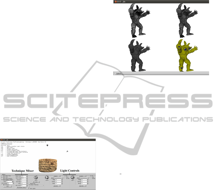
Figure 3: User Interface: Allows user to set light to
achieve maximum entropy and linearly combine different
techniques by assigning them weights and then clicking on
“Recompute Colors”
The light and view direction vectors are uniformly
distributed over the surface of a unit sphere centered
at the origin. To cover the range of possible com-
binations of light and view directions, we render the
models while varying these directions over a uniform
sampling of the unit sphere. The light is positioned in
order to maximize entropy.
3.3.1 Smoothing
We do not expect the trainer to be a visualization ex-
pert, but rather a domain expert or even a novice user.
Furthermore, since the training data is manually gen-
erated and the process can take an hour or even more,
it is possible to generate conflicting training data. In
particular, for the same or similar features multiple
Figure 4: Feature Selection User Interface with Test Object:
Four different renderings can be viewed, bottom right shows
blue selected vertices.
techniques may be chosen over the course of the train-
ing. To ensure consistency, we employ a smoothing
pass to the data. This is done by assigning weights
to the feature-technique correspondence. For exam-
ple, if the same feature occurs twice in the training-set
with different learned scalars, we reduce the weight of
each rule symmetrically so that they sum to 1.0. We
further use a similarity threshold ε to ensure that sim-
ilar features with differing rules have proportionally
reduced confidence. A function that achieves this is
as follows. For a feature f if there exists a set of other
features { f
i
},1 ≤ i ≤ k such that d
i
= | f − f
i
| < ε,
where | | denotes the L
1
norm, we assign f a weight
w =
1
k
+
∑
d
i
.
3.3.2 Learning and Prediction
We have used Support Vector Machines (SVM) pro-
vided in libSVM (Chang and Lin, 2011) for regres-
sion and classification.
In our regression approach, the intensity (I) at
a vertex is assumed to be a function (f ) of the
vertex feature vector (v), i.e., I = f (v) where I ∈
[0,1] , v = {θ, φ,c
1
,c
2
,o} ∈ R
5
and f : R
5
→ [0, 1]
in the basic feature vector case, for example.
A plot of the feature space is shown in Figure 5
which suggests a linear model may be sufficient. We
use ε-SVR (Support Vector Regression (Chang and
Lin, 2011)) to estimate the linear function f. For each
visible vertex of the 3D model to be visualized, an in-
tensity value is predicted by the SVM. At the render-
ing time, the base diffuse component of each vertex
is scaled by this intensity value to produce the visual-
ization.
We also employ a simplified classification only
approach, where only the best suited technique for a
User-guidedModulationofRenderingTechniquesforDetailInspection
251

Figure 5: Feature Space of Learning Data Set for Armadillo
model (see Figure 4): The three axes are the principal cur-
vatures c
1
, c
2
and the θ, the angle between the light direc-
tion and the surface normal. The color of a feature point
corresponds to a particular intensity.
given model is predicted. In other words, only one
of the scalars is allowed to be 1.0 and the others set
to 0. For this classification, we employ C-SVC (Sup-
port Vector Classifiers (Chang and Lin, 2011)) rather
than the regression. The technique number (T, refer
Table 1) is the class label. The classifier provides a
function (f ) that gives the class number for a vertex
feature vector, i.e., T = f (v) where T ∈ {1..7} , v =
{θ,φ, c
1
,c
2
,o} ∈ R
5
and f : R
5
→ {1..7}.
At the rendering time, the technique number is
computed for each visible vertex of the 3D model and
the final color is computed accordingly.
3.4 Results
For the first experiment, we use the canonical test
objects (see Figure 6) to obtain the dataset with the
standard vertex feature vector. Only mean curvature
shading and diffuse lighting are used. Figure 6 shows
3 views that produce high entropies with the light
placed directly pointing into the plane of the paper.
Figure 6: Simple Test Object: Mean Curvature Shading and
Diffuse Lighting.
The regression approach is then applied to obtain
a visualization of the Armadillo model (shown in Fig-
ure 7).
For the second experiment, the trainer selects parts
of the test model that appear better with a partic-
ular technique. The test model is the Armadillo
shown in Figure 4. All three techniques viz. diffuse
lighting, mean curvature shading, ambient occlusion
and their combinations are explored (refer Table 1).
Figure 7: Regression Based Approach Results for Ar-
madillo 3D Model. Four renderings are shown, separating
the left and the right halves for better comparison: from the
left – Ambient Occlusion, Our Approach, Diffuse Lighting
and Mean Curvature Shading. Training set is derived from
canonical models as shown in Figure 6.
Classification based learning approach is used. The
learned scalar values are then applied to visualize the
Cuneiform Tablet as shown in Figure 8.
Figure 8: Classification Approach Results for Cuneiform
Tablet 3D Model: Our approach (top left), Ambient Occlu-
sion (top right), Diffuse Lighting (bottom left), Mean Cur-
vature Shading (bottom right). Training data obtained from
Armadillo model in Figure 4.
Table 2 lists the time taken to predict vertex color
values using the two approaches.
Table 2: Results: Time taken vs number of vertices in 3D
model and number of feature vectors in training data set.
The number of Support Vectors (SV) is also listed.
Training
Dataset
Size
Num
of
SV
Number
of Ver-
tices
Time(s)
Regression
(Fig. 7)
310005 297775 172974 874
Classification
(Fig. 8)
1015 694 1861168 39
We next repeat the second experiment using the
augmented vertex feature vector. The light position is
GRAPP2014-InternationalConferenceonComputerGraphicsTheoryandApplications
252
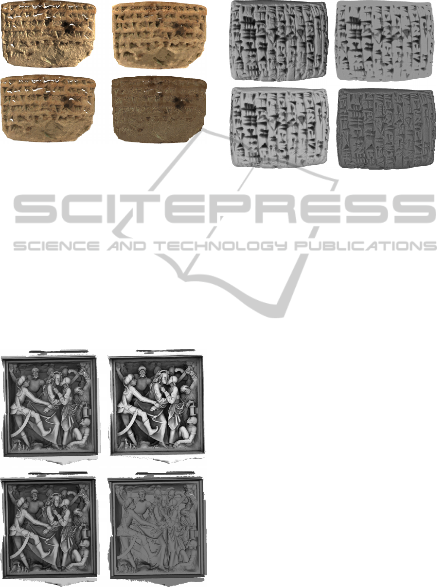
Figure 9: Classification using Augmented Feature Vector
applied to Cuneiform2. We have applied the scalars learned
from the Armadillo model (Figure 4) to visualize three dif-
ferent models. Four images are shown for each model (two
in the next two figures). Our approach is used for each im-
age on the top left, Ambient Occlusion is used on the top
right, Diffuse Lighting+AO+Mean Curvature on the bottom
left, and Mean Curvature Shading on bottom right.
learned via entropy maximization. The visualizations
are shown in Figures 9 to 11.
We can see that even though the individual steps
of our technique can be improved, the visualizations
it produces are meaningful. Augmented feature vec-
tor generally outperforms the basic vector. An infor-
mal study of ten graduate students is indicative of the
method’s perceptual effectiveness. Seven renderings
Figure 10: Classification using Augmented Feature Vector
applied to 3D Mural. Our approach is on top left.
Figure 11: Classification using Augmented Feature Vector
applied to Cuneiform3. Our approach is on top left.
of four models (three Cuneiform tablets and one Mu-
ral) were shown to each user. Seven were chosen from
the library of techniques and one was the results of the
learned technique. They were asked to assign a score
between 1 and 5 to each. Although the learned tech-
nique did not score the highest mark in each of the 40
cases, it was ranked the highest in 31 cases.
4 CONCLUSION AND FUTURE
WORK
We propose a novel way to inspect cultural artifacts
with the aid of machine-learning techniques. An auto-
mated approach to combine multiple rendering tech-
niques has been presented. The approach is promis-
ing: as the survey shows, a per-vertex combination
of rendering techniques can outrank each individual
component applied globally in a model. Further, the
weights of basis techniques vary substantially from
vertex to vertex. It is hard to choose this manually
on a per vertex basis. Our approach uses supervised
machine learning to learn users’ preferences and pre-
dict shading values for new models. The advantages
of this approach are:
• Using only a few test models, the approach gives
reasonably good results for new models.
• The technique can capture non-local context as
the users’ notion of a good rendering is based on
the overall perception of the complete model.
• Due to per-vertex computations being carried out,
each part of the model gets optimally shaded for
each view configuration.
User-guidedModulationofRenderingTechniquesforDetailInspection
253

Our results show that learning based visualization
is a promising approach, even if the technique learned
by our current algorithm is not always the best in
our experiments. We have presented only early re-
sults and there is much scope for further study in
this direction. There is a need for to devise a theo-
retical framework for determining useful parameters
to learn. Algorithmic work is also required to al-
low faster computation of view-dependent training re-
sults for interactive manipulation. Also, other render-
ing techniques like specular lighting and cast shadows
could be added to the learning set. A more efficient
training set generation would also be useful in making
the technique user friendly.
ACKNOWLEDGEMENTS
We thank the Department of Science and Technology
for funding this research and Lissy Verma for imple-
menting several basis rendering techniques. We also
thank the reviewers for helping improve the presenta-
tion of the paper.
REFERENCES
Anderson, S. and Levoy, M. (2002). Unwrapping and vi-
sualizing cuneiform tablets. Computer Graphics and
Applications, IEEE, 22(6):82 – 88.
Bartz, D., Hagen, H., Interrante, V., Ma, K.-L., and Preim,
B. (2005). Illustrative rendering techniques for visu-
alization: Future of visualization or just another tech-
nique? In Visualization, 2005. VIS 05. IEEE, pages
715–718.
Cavanagh, P. and Leclerc, Y. (1989). Shape from shadows.
Journal of Experimental Psychology: Human Percep-
tion and Performance, 15:13–27.
Chang, C.-C. and Lin, C.-J. (2011). Libsvm: A library
for support vector machines. ACM Trans. Intell. Syst.
Technol., 2(3):27:1–27:27.
Cignoni, P., Scopigno, R., and Tarini, M. (2005). A
simple normal enhancement technique for interactive
non-photorealistic renderings. Computer & Graphics,
29(1):125–133.
Costa, A. C., De Sousa, A. A., and Ferreira, F. N. (1999).
Lighting design: A goal based approach using opti-
mization. In Lischinski, D. and Larson, G. W., editors,
Rendering Techniques, pages 317–328. Springer.
Deussen, O., Hiller, S., van Overveld, C., and Strothotte,
T. (2000). Floating points: A method for computing
stipple drawings. Computer Graphics Forum, 19:40–
51.
Gumhold, S. (2002). Maximum entropy light source place-
ment. In Visualization, 2002. VIS 2002. IEEE, pages
275 –282.
Halle, M. and Meng, J. (2003). Lightkit: a lighting system
for effective visualization. In Visualization, 2003. VIS
2003. IEEE, pages 363 –370.
Jolivet, V., Plemenos, D., and Poulingeas, P. (2002). Inverse
direct lighting with a monte carlo method and declar-
ative modeling. In Proceedings of the International
Conference on Computational Science-Part II, ICCS
’02, pages 3–12, London, UK, UK. Springer-Verlag.
Kindlmann, G., Whitaker, R., Tasdizen, T., and M
¨
oller,
T. (2003). Curvature-based transfer functions for di-
rect volume rendering: Methods and applications.
In Proceedings of the 14th IEEE Visualization 2003
(VIS’03), VIS ’03, pages 67–, Washington, DC, USA.
IEEE Computer Society.
Langer, M. S. and B
¨
uLthoff, H. H. (2000). Depth discrim-
ination from shading under diffuse lighting. Percep-
tion, 29(6):649–660.
Poulin, P. and Fournier, A. (1992). Lights from highlights
and shadows. In Proceedings of the 1992 symposium
on Interactive 3D graphics, I3D ’92, pages 31–38,
New York, NY, USA. ACM.
Poulin, P., Ratib, K., and Jacques, M. (1997). Sketching
shadows and highlights to position lights. In Proceed-
ings of the 1997 Conference on Computer Graphics
International, CGI ’97, pages 56–, Washington, DC,
USA. IEEE Computer Society.
Rusinkiewicz, S., Burns, M., and DeCarlo, D. (2006).
Exaggerated shading for depicting shape and detail.
ACM Trans. Graph., 25(3):1199–1205.
Takahashi, S., Fujishiro, I., Takeshima, Y., and Nishita, T.
(2005). A feature-driven approach to locating optimal
viewpoints for volume visualization. In Visualization,
2005. VIS 05. IEEE, pages 495 – 502.
V
´
azquez, P.-P. and Sbert, M. (2003). Perception-based il-
lumination information measurement and light source
placement. In Proceedings of the 2003 international
conference on Computational science and its appli-
cations: PartIII, ICCSA’03, pages 306–316, Berlin,
Heidelberg. Springer-Verlag.
Vergne, R., Pacanowski, R., Barla, P., Granier, X., and
Shlick, C. (2011). Improving shape depiction under
arbitrary rendering. IEEE Transactions on Visualiza-
tion and Computer Graphics, 17(8):1071–1081.
Wang, C. and Shen, H.-W. (2011). Information theory in
scientific visualization. Entropy, 13(1):254–273.
Wang, S., Cai, K., Lu, J., Liu, X., and Wu, E. (2010). Real-
time coherent stylization for augmented reality. The
Visual Computer, 26(6-8):445–455.
GRAPP2014-InternationalConferenceonComputerGraphicsTheoryandApplications
254
