A Bayesian Framework for Enhanced Geometric Reconstruction of

Complex Objects by Helmholtz Stereopsis

Nadejda Roubtsova and Jean-Yves Guillemaut

Centre for Vision, Speech and Signal Processing, University of Surrey, Guildford, U.K.

Keywords:

3D Reconstruction, Helmholtz Stereopsis, Complex Reﬂectance

Abstract:

Helmholtz stereopsis is an advanced 3D reconstruction technique for objects with arbitrary reﬂectance proper-

ties that uniquely characterises surface points by both depth and normal. Traditionally, in Helmholtz stereopsis

consistency of depth and normal estimates is assumed rather than explicitly enforced. Furthermore, conven-

tional Helmholtz stereopsis performs maximum likelihood depth estimation without neighbourhood consid-

eration. In this paper, we demonstrate that reconstruction accuracy of Helmholtz stereopsis can be greatly

enhanced by formulating depth estimation as a Bayesian maximum a posteriori probability problem. In re-

formulating the problem we introduce neighbourhood support by formulating and comparing three priors: a

depth-based, a normal-based and a novel depth-normal consistency enforcing one. Relative performance eval-

uation of the three priors against standard maximum likelihood Helmholtz stereopsis is performed on both

real and synthetic data to facilitate both qualitative and quantitative assessment of reconstruction accuracy.

Observed superior performance of our depth-normal consistency prior indicates a previously unexplored ad-

vantage in joint optimisation of depth and normal estimates.

1 INTRODUCTION

As evidenced by the formidable volume of past and

active research, reconstruction of 3D geometry is both

challenging and much desirable for practical applica-

tions. A tremendous progress has been made in the

ﬁeld with sub-millimetre accurate geometries being

obtained when capture conditions and surface prop-

erties are tailored for reconstruction. All prior al-

gorithms rely on multiple images to resolve inherent

depth ambiguity, while differing in acquisition and

view correlation employed to formulate ambiguity re-

solving constraints. Also variable is the degree of

neighbour support used when characterising a surface

point by its depth, normal or both.

The oldest of 3D reconstruction techniques

is conventional stereopsis thoroughly surveyed in

(Scharstein and Szeliski, 2002) and (Seitz et al., 2006)

for single- and multi-view respectively. Conventional

stereopsis computes disparity through feature-point

intensity matching between acquired views in the

presence of sufﬁcient texture. In this approach, sur-

face points are characterised by depth, which is re-

ciprocal to disparity. Conventional intensity-based

stereo strongly relies on the inter-viewpoint constancy

of feature appearance (i.e. Lambertian reﬂectance)

failing when the assumption is violated. Alternative

SIFT features are robust to intensity variations, al-

though they only facilitate sparse representation.

Another reconstruction approach called photo-

metric stereopsis (Woodham, 1989) permits an arbi-

trary reﬂectance model as long as it is a priori known.

Photometric constraints are linked to the response of a

point to varying illumination at a constant viewpoint.

The sought surface orientation is the one best recon-

ciling intensity predictions and measurements. Essen-

tially, the reﬂectance issue of conventional stereo is

not solved by photometric stereo but rather the bur-

den of it is shifted to the calibration phase of which

a surface-orientation-dependent reﬂectance model is

required. Reﬂectance modelling is a tedious task, of-

ten impossible to the desired accuracy for real objects.

With an accurate model, photometric stereo directly

outputs highly descriptive surface normals. Individual

normals however need to be integrated into a surface

often resulting in drift (global shape distortion) due to

accumulation of numerical integration errors. Unlike

conventional stereo, photometric stereo with its single

viewpoint avoids the task of feature-point matching.

There are few techniques bypassing the need for

reﬂectance modelling. One old example is the shape-

from-silhouette algorithm (Baumgard, 1974) which

335

Roubtsova N. and Guillemaut J..

A Bayesian Framework for Enhanced Geometric Reconstruction of Complex Objects by Helmholtz Stereopsis.

DOI: 10.5220/0004683503350342

In Proceedings of the 9th International Conference on Computer Vision Theory and Applications (VISAPP-2014), pages 335-342

ISBN: 978-989-758-009-3

 2014 SCITEPRESS (Science and Technology Publications, Lda.)

computes a rough 3D outline of the object, its visual

hull (Laurentini, 1994), by intersecting visual cones

of multiple views. Visual hull is used for initialisa-

tion by many advanced reconstruction algorithms. A

more recent highly promising photometric technique

of Helmholtz stereopsis (HS) (Zickler et al., 2002) ad-

dresses the fundamental problem of reﬂectance mod-

elling by enforcing consistency of reﬂectance-model-

independent Helmholtz reciprocity observation: i.e.

swapping the sensor and the light source does not alter

reﬂectance response. Besides its independence of the

reﬂectance model, HS has the unique feature of point

characterisation by both depth and normal. However,

in its conventional formulation, HS is sequential with

depth estimates uniquely determining the normals.

Such unidirectional indexation of normals by depth

estimates means that the typically noisy HS depth

maps result in normal inaccuracies and hence in local

and global reconstruction errors (although a certain

degree of robustness to normal errors has been ob-

served). Conceptually, the depth-normal dependency

need not be unidirectional: depth and normal estima-

tion can be uniﬁed in a single framework enforcing

consistency and comparable accuracy levels of both

estimates.

Conventional HS essentially performs maximum

likelihood estimation (MLE). Even in the absence of

noise, inherent point depth ambiguities exist, for in-

stance, due to coincidental symmetries in the acquisi-

tion set-up conﬁguration relative to the sampled sur-

face. Since local evidence is ambiguous, neighbour-

hood support is clearly needed and warranted as there

is always a degree of local smoothness in real objects.

Yet, to our knowledge, MAP optimisation in the con-

text of HS has not been previously attempted. In this

paper, we propose a novel MAP formulation embed-

ding HS into a Bayesian framework with a prior that

for the ﬁrst time explicitly enforces consistency be-

tween depth and normals. We show that, with the con-

sistency prior, MRF optimisation of MAP HS indeed

results in superior reconstruction accuracies. Un-

like alternative depth-based or normal-based priors,

the depth-normal consistency prior capitalises on the

unique ability of HS to provide both depths and nor-

mals and, combining the two, produces the most cor-

rect geometries coherent in both depth and integrated

normal representation. These conclusions are based

on the quantitative and qualitative evaluation compar-

ing conventional ML HS to MAP optimisation with 1.

classical depth-based; 2. normal-based and 3. novel

depth-normal consistency priors.

2 RELATED WORK

Helmholtz reciprocity states that a light ray and its re-

verse will undergo the same processes of reﬂection,

refraction and absorption (Helmholtz, 1925). Let ˆv

be the unit vector directed from the surface point to

the camera and ˆv

the corresponding vector from the

surface point to the light source. The implication

of Helmholtz reciprocity, ﬁrst observed by Zickler

et al. (Zickler et al., 2002) in the context of multi-

view reconstruction, is that interchanging the light

source and camera in the set-up, thereby swapping

the vector deﬁnitions, has no effect on the point’s re-

ﬂective behaviour. Mathematically, Bidirectional Re-

ﬂectance Distribution Function (BRDF) f

is recipro-

cal: f

( ˆv

, ˆv

) = f

( ˆv

, ˆv

). The following standard

image formation equations for reciprocal images I

and I

respectively:

= f

( ˆv

, ˆv

)

ˆn · ˆv

, i

= f

( ˆv

, ˆv

)

ˆn · ˆv

(1)

express a surface point’s image intensities i

and i

a function of BRDF, surface normal ˆn, the two recip-

rocal unit vectors and the radiation fall-off factor r.

Reciprocity of BRDF in conjunction with Equation 1

result in the following constraint ˆw notably without

any dependency on the BRDF:



ˆv

− i

ˆv



· ˆn = ˆw · ˆn = 0. (2)

With a single ˆw per reciprocal pair, 3 or more re-

ciprocal pairs result in constraint matrix W to which

singular value decomposition (SVD) can be applied:

SV D(W ) = U ΣV

∗

where U,V are unitary and Σ is a

rectangular diagonal matrix. The last column of V

gives the normal at the sampled point. The last diag-

onal value of Σ, the SVD residual σ

, tends to 0 when

there is a mutual constraint consistency. For outlier

elimination, Zickler et al. also involve σ

in their con-

sistency measure: the SVD coefﬁcient

σ2

σ3

tends to in-

ﬁnity for consistent W (those of true surface points).

The requirement of multiple reciprocal pairs and

the need for careful ofﬂine calibration led to discus-

sions on acquisition impracticality of HS. In response,

Zickler in (Zickler, 2006), ﬁrstly, devises an auto-

calibration algorithm using specular highlights and

intensity patches, two inherent easily identiﬁable re-

gions of interest. Unlike conventional stereo, inten-

sity matching in HS is not conditional on the valid-

ity of the Lambertian assumption making intensity

patches stable calibration markers.

The inherent appearance predictability of an in-

tensity patch of one reciprocal image based on the

other is also employed in (Tu et al., 2003) to formu-

late prediction error for registration in full 3D HS.

VISAPP2014-InternationalConferenceonComputerVisionTheoryandApplications

336

Work on full 3D HS is scarce. The work of De-

launoy et al. (Delaunoy et al., 2010) and the more re-

cent publication of Weinmann et al. (Weinmann et al.,

2012) are two notable examples. Both are variational

approaches requiring computationally intensive opti-

misation over the entire surface with long execution

times. The method of Weinmann et al. is more cum-

bersome due to fusion with structured light at acquisi-

tion. The impracticalities are however outweighed by

the impressive degree of demonstrated reconstruction

detail.

To address the issue of multiple constraint require-

ment, Zickler et al. in (Zickler et al., 2003) propose

binocular HS i.e reconstruction from a single recipro-

cal pair. The method is a differential approach where

the (single) constraint is formulated as a PDE of depth

over the surface coordinates. The PDE requires ini-

tialisation and results in a family of solutions the am-

biguity of which is resolved through multi-pass op-

timisation. Although interesting as an exercise on

acquisition simpliﬁcation, additional computational

complexity is perhaps not outweighed by the advan-

tages.

Binocular HS and full 3D HS methods exploit

the advantages of optimisation over a set of sur-

face points. In the original HS, the depth label at

each point is computed independently of its neigh-

bours (without a Bayesian prior). Logically, there

is a strong correlation between neighbouring surface

points. By formulating a prior, the problem is turned

into a MAP one, solvable by numerous mature MRF

optimisation techniques (Szeliski et al., 2008). The

value of MRF optimisation for other 3D reconstruc-

tion approaches has been established. In conventional

stereo, the top-performers are global optimisation al-

gorithms solved through MRF-based graph-cuts and

belief propagation (Scharstein and Szeliski, 2002).

(Wu et al., 2006) is an interesting work where MRF

optimisation is performed in the context of photo-

metric stereo with a normal-based (rather than depth-

based) prior achieving remarkable robustness in the

face of noisy input, complex geometries, shadows,

transparencies etc..

Conventional HS will similarly beneﬁt from

MRF-based optimisation, since geometries obtained

by ML HS lack in smoothness and ﬁne structural

detail due to inherent depth ambiguities, intensity

measurement noise, sensor saturation and calibra-

tion/discretisation errors. Aimed at tackling the issues

of conventional HS, the contributions of this paper are

twofold. Firstly, we devise a MAP framework allow-

ing to apply MRF-based optimisation in the context of

HS. Secondly, we introduce a novel smoothness prior

enforcing coherence of depth and normal estimates of

HS and show superiority of the prior over the purely

depth-based or normal-based ones.

3 METHODOLOGY

In reconstruction by HS, we begin with N recipro-

cal image pairs (N ≥ 3) and a discrete volume V

of N

× N

voxels v(x, y, z) containing the ob-

ject. Each v(x, y, z) is sampled by projection onto

the reciprocal images to acquire a set of N intensity

2-tuples

{

, i

)

, .., (i

, i

)

}

and formulate N con-

straints ˆw as in Equation 2. Only those v(x, y, z) ∈

V containing surface points will have N mutually

consistent constraints. In standard HS, voxel sets

p(x,y)

= {v(x, y, z) : x = x

∗

, y = y

∗

} with constant

2D coordinates x

∗

and y

∗

are sampled exhaustively

over V . Each R

p(x,y)

deﬁnes the depth search space

for random variable p(x, y) with the optimal depth

value z

p(x,y)

= z

∗

p(x,y)

corresponding to the surface

point P(x, y, z

∗

p(x,y)

). In our work, the object’s vi-

sual hull (VH) restricts the search space to R

V H

p(x,y)

{v(x, y, z) : x = x

∗

, y = y

∗

, v(x

∗

, y

∗

, z

p(x,y)

) ∈ V H} (im-

plicit in Equations 4 and 5) limiting sampling in both

2D ( R

p(x,y)

∩V H =

0 for some p(x, y)) and depth.

We postulate that depth estimation of HS is in

fact a labelling problem where each random variable

p(x, y) is assigned depth label z

∗

p(x,y)

. The optimal

solution to such a labelling problem is known (Li,

1994) to be one maximising the a posteriori probabil-

ity (MAP) i.e. the likelihood of a parameter assum-

ing a certain value given the observation. The prob-

lem is typically translated into the equivalent one of

posterior energy minimisation where the total energy

is a sum of likelihood (data) and prior energy terms.

Likelihood is related to the noise model of the obser-

vation representing its quality, viewed independently

of the other observations. The prior term (typically lo-

cal smoothness) is the knowledge of the problem en-

capsulating interaction between observations. In our

work, the interaction is contained within the Marko-

vian neighbourhood of p(x, y) restricted by VH:

N (p(x, y)) = {p(x + k, y + (1 − k)) :

k ∈ {0, 1}, R

V H

p(x+k,y+(1−k))

0} (3)

In this paper, we formulate depth estimation of HS

as a MAP problem in Equation 4. For each ran-

dom variable p(x, y) and given p(x

, y

) ∈ N (p(x, y)),

we deﬁne normalised data and smoothness costs,

(x, y, z

p(x,y)

) and E

(x, y, z

p(x,y)

, x

, y

, z

p(x

)

) re-

spectively, weighted by the normalised parameter α.

The total optimisation is over all random variables

within VH. The solution to the labelling problem is

ABayesianFrameworkforEnhancedGeometricReconstructionofComplexObjectsbyHelmholtzStereopsis

337

the label conﬁguration f

∗

= {z

∗

p(x,y)

∈ [Z

, .., Z

] : x ∈

, .., X

], y ∈ [Y

, ..,Y

]} selected from a set of S

such conﬁgurations.

∗

MAP

= argmin

f ∈S

∑

p(x,y)

((1 − α)E

(x, y, z

p(x,y)

) +

∑

p(x

)∈N (p(x,y))

αE

(x, y, z

p(x,y)

, x

, y

, z

p(x

)

)) (4)

In contrast to our approach, conventional HS solves a

simpler maximum likelihood (ML) optimisation prob-

lem, without the smoothness prior, resulting a sub-

optimal solution because each random variable is op-

timised independently:

∗

= argmin

f ∈S

∑

p(x,y)

(x, y, z

p(x,y)

) (5)

Sub-optimality leads to noisy depth maps and hence

lacking surface smoothness and structural detail. The

global shape may be reasonable, but the recon-

struction ﬁnesse of conventional HS is limited be-

cause noisy depth labels index approximate normals.

Through Bayesian formulation in Equation 4, we en-

deavour to obtain cleaner depth maps improving accu-

racy by more accurate normal indexing. A Bayesian

framework is clearly more suitable because of the

strong statistical dependency between neighbouring

depth estimates. The following sections deﬁne data

energy and three investigated smoothness priors.

3.1 Data Term

Depth hypothesis z of each p(x, y) has got a likeli-

hood E

(x, y, z) deﬁned through the SVD coefﬁcient

(v(x,y,z))

associated with the corresponding voxel.

The coefﬁcient tends to inﬁnity as z approaches the

correct depth z

∗

. Since MRF optimisation is formu-

lated as a minimisation, E

(x, y, z) is a decaying func-

tion of

(v(x,y,z))

. Throughout the paper, we adhere

to the exponential formulation with the decay factor

µ = 0.2 × log(2):

(x, y, z) = e

−µ×

(v(x,y,z))

(6)

As it indicates likelihood, the function is bounded in

the range [0, 1].

3.2 Smoothness Term

Unlike conventional data-based HS, we introduce

priors. We devise three prior types reﬂecting the

unique ability of HS to generate both depth and nor-

mal estimates.

1. Depth-based Prior. The prior is known from

conventional stereo. In this work, we deﬁne depth-

based smoothness cost E

s d

(x, y, z, x

, y

, z

) of voxel

v(x, y, z) relative to v(x

, y

, z

) by the discontinuity-

preserving truncated squared difference of the neigh-

bouring depth hypotheses normalised by the total

number of labels (N

s d

(x, y, z, x

, y

, z

) = λ × min(S

max

, (z − z

)

) (7)

where S

max

= (0.5 × N

)

is the truncation value and

λ = (N

)

−2

is the normalising constant. With penal-

ties for much different labels at neighbouring sur-

face points, the prior encourages piece-wise constant

depth and biases towards a fronto-parallel represen-

tation. Discontinuities are preserved by truncation

moderating depth ﬂuctuation penalties.

2. Normal-based Prior. Surface characterisation

through normals is typical of photometric techniques.

A suitable normal-based prior would enforce locally

constant normals encouraging locally ﬂat, though not

necessarily fronto-parallel, surfaces. Hence, this prior

is less restrictive of reconstructed surfaces than the

depth-based one. The complication in formulating

normal-based priors arises because 1. normals are

continuous 3D quantities that cannot be labels in our

discrete framework and 2. normal correlations are

irregular expressions not optimisable by graph cuts

(Kolmogorov and Zabih, 2004). In this work, dis-

crete depths are still the labels, but rather than depth

information, we use the corresponding normal sim-

ilarity to assess label compatibility. Sequential tree

re-weighted message passing (TRW-S) (Wainwright

et al., 2005), (Kolmogorov, 2006) MRF optimisation

is used consistently throughout the paper because it

does not require regularity of prior.

Given photometric normal ˆn(x, y, z) =

, n

)> and ˆn(x

, y

, z

) = (n

, n

)> of

voxels v(x, y, z) and v(x

, y

, z

) respectively, we

formulate the smoothness-based constraint:

s n

(x, y, z, x

, y

, z

) =

−1

arccos



ˆn(x, y, z) · ˆn(x

, y

, z

)



(8)

The cost function of Equation 8 is the normalised

correlation angle between normals.

3. Depth-normal Consistency Prior. The depth-

based prior seeks to clean up depth maps by enforcing

their smoothness, while the normal-based approach

promotes gradual spatial evolution of the normal ﬁeld.

Both approaches are one-sided: the depth is optimised

indexing the normals or vice versa. Depth and nor-

mal estimation processes are however not indepen-

dent and must be consistent with each other. We

formulate a prior explicitly enforcing consistency be-

tween depths and normals, for the ﬁrst time perform-

ing joint depth map and normal ﬁeld optimisation.

VISAPP2014-InternationalConferenceonComputerVisionTheoryandApplications

338

Figure 1: Real data: object appearance.

Each depth transition between v(x, y, z) and

v(x

, y

, z

) uniquely deﬁnes local geometric normal

ˆn

(x, y, z, x

, y

, z

), always contained in the transition

plane (xz or yz). If the depth transition is correct, the

geometric normal correlates well with the projections

of the photometric normals of v(x, y, z) and v(x

, y

, z

)

(their normal estimates), respectively ˆn

ph pr j

(x, y, z)

and ˆn

ph pr j

, y

, z

), onto the corresponding depth

transition plane. Mathematically, the correlation de-

gree can be expressed by the correlation angle. For

example, for v(x, y, z) we have:

ph−g

= π

−1

arccos( ˆn

ph pr j

(x, y, z) · ˆn

(x, y, z, x

, y

, z

))

(9)

Since the range of the arc-cosine function is [0, π], the

orientation of the geometric normal must be forced to

be consistent with the photometric normals (i.e. out of

the surface, z > 0). Hence, the depth-normal consis-

tency prior E

s dn

(x, y, z, x

, y

, z

) is formulated as fol-

lows:

s dn

(x, y, z, x

, y

, z

) =

(φ

ph−g

+ φ

ph−g

) (10)

4 EVALUATION

We perform evaluation of the proposed method on

both real and synthetic data to enable qualitative and

quantitative analysis. Throughout, our method with

its 3 prior options is compared against the standard

HS approach without MRF optimisation. For real

data, the quality of results is assessed visually as there

is no ground truth. Synthetic input imagery, on the

other hand, is generated from an a priori known mesh

and hence permits quantitative assessment of both lo-

cal and global shape deviations of the reconstructions.

4.1 Real Data

Real data is composed of 4 sets (Figure 1) from

(Guillemaut et al., 2008), each posing different chal-

lenges. The billiard ball and the teapots are specular

smooth objects. The teapots are more complex with

wider specularities and 2D texture (e.g. stripes, ﬂow-

ers). The terracotta doll is Lambertian but has many

ﬁne geometric details (e.g. dimples, clothing).

Figure 2 contrasts estimated depth maps and the

corresponding integrated surfaces of the proposed

MAP HS formulation against standard (ML) HS.

MAP optimisation priors are compared by qualita-

tively accessing both local and global accuracy of

the generated depth maps and surfaces. The relative

weight α is tuned for each prior independently but the

optimal setting per prior tends to be consistent across

all datasets. Surface integration is performed from

the normal ﬁelds in the frequency domain using the

Frankot-Chellappa (FC) algorithm (Frankot and Chel-

lappa, 1988).

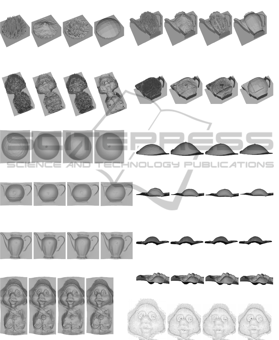
The results in Figure 2 show that, relative

to ML HS, MAP optimisation clearly produces

smoother reconstructions (teapot/ball surface in Fig-

ures 2(e),(f),(g)) with ﬁner structural detail (the doll’s

dimples/eyebrows in Figure 2(h); the corresponding

normal ﬁelds in Figure 2(m) are rectiﬁed to reveal

structural detail). On the relative performance of the

priors, the key observation is that only the depth-

normal consistency prior generates geometrically cor-

rect depth maps. Global accuracy of the depth-based

prior ranges from poor (ball, Figure 2(a)) to rea-

sonable (teapots, Figures 2(b),(d)) and high (doll,

Figure 2(c)). The depth maps of the depth-based

prior are however universally noisy. Correspond-

ing normal-based prior results are consistently heav-

ily distorted. Correct reconstruction is only possible

from a geometrically (globally and locally) accurate

depth map. While this is evident for the doll dataset,

in other cases distorted depth maps of the normal-

based approach may, in the front view, seem to pro-

duce decent reconstructions (Figures 2(f),(g)). The

deceiving appearance results from optimisation ac-

cidentally ﬁnding well-correlating normals at wrong

depths. These integrate into locally smooth surfaces,

yet distort the global shape for all four datasets (Fig-

ures 2(i),(j),(k),(l)). As the depth map accuracy as-

sessment suggests, the best global shape reconstruc-

tion belongs to the depth-normal consistency prior op-

timisation.

HS is known (Guillemaut et al., 2004) to be sensi-

tive to calibration and discretisation errors whereby,

due to projection mismatches, intensity measure-

ments i

and i

within a reciprocal pair are inconsis-

tent. The grave form of inconsistency when, within

a single reciprocal pair, a point is projected into dif-

ferent intensity ﬁelds, results in reconstruction of 2D

(imprinted) texture as geometric detail. Along with

sharpening true geometries, optimisation is seen to

strengthen the effect of calibration errors: e.g. printed

stripes and ﬂowers on the teapots (Figure 1) appear

embedded into geometry (Figure 2(f),(g)). Perform-

ing patch-based intensity averaging during input data

ABayesianFrameworkforEnhancedGeometricReconstructionofComplexObjectsbyHelmholtzStereopsis

339

(a) depth maps, α

= 0.9, α

= 0.1, α

= 0.8 (b) depth maps, α

= 0.9, α

= 0.5, α

= 0.8

= 0.9, α

= 0.5, α

= 0.8

(d) depth maps, α

= 0.9, α

= 0.5, α

= 0.8

(e) FC reconstruction, front view, α

= 0.9, α

= 0.1, α

= 0.8

(f) FC reconstruction, front view, α

= 0.9, α

= 0.5, α

= 0.8

(g) FC reconstruction, front view, α

= 0.9, α

= 0.5, α

= 0.8

(h) FC reconstruction, front view, α

= 0.9, α

= 0.5, α

= 0.8

(i) FC reconstruction, side view, α

= 0.9, α

= 0.1, α

= 0.8

(j) FC reconstruction, bottom view, α

= 0.9, α

= 0.5, α

= 0.8

(k) FC reconstruction, bottom view, α

= 0.9, α

= 0.5, α

= 0.8

(l) FC reconstruction, side view, α

= 0.9, α

= 0.5, α

= 0.8

(m) Normal ﬁelds (doll), α

= 0.9, α

= 0.5, α

= 0.8

Figure 2: Depth maps, normal ﬁelds (doll) and ﬁnal reconstruction by integration using the FFT-based Frankot-Chellappa (FC)

algorithm. In each sequence of 4 images (left to right) standard (ML) HS is compared against proposed MAP HS formulation

using MRF optimisation with depth-based (d), normal-based (n) and depth-normal consistency (dn) priors (data-smoothness

weighting α as indicated in each case). Sampling resolution ∆x × ∆y × ∆z and sampled volumes |V | = N

× N

are as

follows. Doll: 1.0mm ×1.0mm×0.5mm, |V | = 160×82 ×60; teapot no.1: 1.0mm × 1.0mm×0.25mm, |V | = 150×200 × 320;

teapot no.2: 1.0mm × 1.0mm × 0.25mm, |V | = 120 × 190 × 480; billiard : 1.0mm × 1.0mm × 0.25mm, |V| = 60 × 60 × 100.

VISAPP2014-InternationalConferenceonComputerVisionTheoryandApplications

340

(a) Improved depth maps (b) Improved FC reconstructions

Figure 3: Mitigation of saturation and mis-calibration artefacts through patch-based averaging. Settings: MAP HS with

depth-normal consistency prior, patch-based averaging and α

= 0.5.

0 0.001 0.002 0.003 0.004 0.005 0.006 0.007 0.008 0.009 0.01

0.005

0.01

0.015

0.02

0.025

0.03

0.035

0.04

0.045

normalised noise variance

RMS geometric error [m]

standard HS

MRF depth−based prior

MRF normal−based prior

MRF depth−normal consistency prior

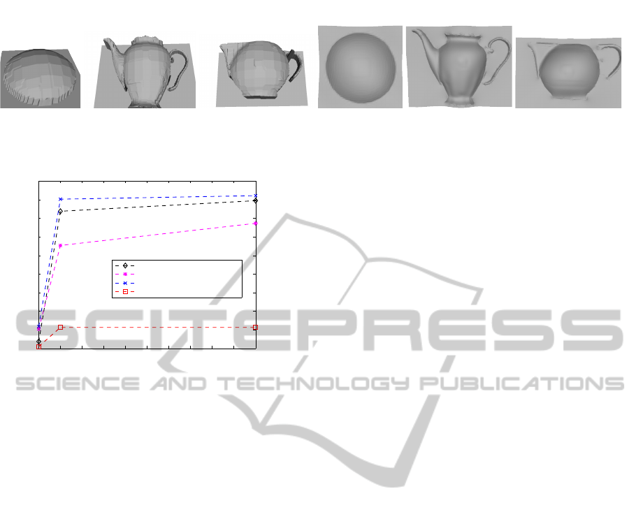
Figure 4: Quantitative evaluation on synthetic data. RMS

geometric error as a function of normalised intensity noise

variance for our MRF (MAP) HS formulation with different

priors and standard (ML) HS.

sampling to bring inconsistent measurements into

closer correspondence would counteract the problem

(Guillemaut et al., 2004). The measure mitigates sat-

uration artefact as well since, instead of the indiscrim-

inative sensor upper limit, the intensities in Equation

2 acquire more meaningful values through regional

support of patch-based averaging. In Figure 3(a) we

show how patch-based averaging effectively elimi-

nates depth errors in the saturated and pattern regions,

hence eliminating/substantially mitigating saturation

and embedded 2D texture artefacts (Figure 3(b)).

4.2 Synthetic Data

Our synthetic object of choice is a sphere (radius =

200 mm). The mesh of the sphere is rendered in

POV-Ray (POV-Ray, 2013) with reﬂectance consist-

ing of diffuse and specular components and under

controlled camera/light source conﬁgurations to pro-

duce 8 noise-free reciprocal pairs. For robustness as-

sessment, two additional image sets are produced by

corrupting the original set by Gaussian zero-mean in-

tensity noise with the variance levels of respectively

0.001 and 0.01. Reconstruction quality is quantiﬁed

by the geometric error: the reconstructed mesh is

sampled for each point seeking the closest distance on

the target ground truth mesh. Figure 4 shows the RMS

error as a function of noise variance comparing stan-

dard ML HS and our MRF (MAP) formulation with 3

different priors (sampled volume |V | = 82 × 82 × 251

at resolution 5mm × 5mm × 1mm). The input inten-

sity range is [0, 65535]. Hence, the normalised noise

variance of 0.001 and 0.01 translates into the abso-

lute intensity standard deviations of 2072 and 6554

respectively. Surface integration is performed us-

ing unscreened Poisson surface reconstruction (Kazh-

dan et al., 2006) because the method outputs surfaces

characterised in the absolute world coordinate system

facilitating their easy comparison unlike FC surfaces

in their individual relative reference frames needing

alignment.

In Figure 4 MRF optimisation with the depth-

normal consistency prior clearly outperforms the

other approaches by an order of magnitude mar-

gin achieving reconstruction accuracies of roughly

0.5mm and 5mm for noise-free and noise-corrupted

sets respectively. The accuracy of the other methods

is the order of a few mm and a few cm for the two

respective cases. For the noise-free case, standard HS

comes closest to the depth-normal prior with the 2mm

error. The second observation to be made is that the

normal-based prior is utterly ineffective with the ac-

curacy always below standard HS, consistent global

shape distortion and the greatest performance deteri-

oration with increased noise levels owing to the high

susceptibility of normals as continuous 3D quanti-

ties to input noise via SVD. Even for the noise-free

case, the error with the normal-based prior is high be-

cause there is no theoretical guarantee that the best

correlating normals correspond to the correct depth

positions. The depth-based prior appears to facilitate

an improvement compared to standard HS for noise-

corrupted data. On visual inspection however, the

depth-based reconstruction is seen to retain the global

shape distortion of the standard HS result, albeit mit-

igated as its lower RMS indicates. In the noisy case,

only our depth-normal consistency prior produces a

global shape visually acceptable as a sphere.

5 CONCLUSIONS

We have proposed a novel MRF optimisable MAP

ABayesianFrameworkforEnhancedGeometricReconstructionofComplexObjectsbyHelmholtzStereopsis

341

formulation of HS, instead of its standard ML form.

To this end, we formulated and compared a depth-

based, a normal-based and a specially tailored depth-

normal consistency prior. We conclude that correctly

utilising the given of piece-wise surface smoothness

in the MAP formulation greatly improves both local

and global reconstruction accuracy relative to ML re-

sults. Both quantitative and qualitative results indi-

cate our depth-normal consistency prior to be the cor-

rect formulation of the smoothness term, which by

enforcing consistency between depth and normal in-

formation produces the best results in terms of both

local smoothness and global object shape. The re-

sults generated with the prior are uniquely consistent

in both depth and integrated normal domain with the

normals being indexed from a geometrically correct

depth map. The computational overhead for the prior

is dependent on the size of the sampled voxel volume

and for the presented real data ranges from 2 min-

utes (billiard ball) to 4 hours (teapot no. 2). In our

future work we are conﬁdent the run-times will be re-

duced substantially by embedding MRF optimisation

of Bayesian HS into a coarse-to-ﬁne framework using

octrees and/or by parallelising and porting prior cost

pre-computation (the bottleneck of the pipeline) onto

the GPU. In addition, we shall explore the potential

of our MRF framework in resolving ambiguities in

the sensor saturation region and at grazing sampling

angles.

REFERENCES

Baumgard, B. (1974). Geometric Modeling for Computer

Vision. PhD thesis, University of Stanford.

Delaunoy, A., Prados, E., and Belhumeur, P. (2010). To-

wards full 3D Helmholtz stereovision algorithms. In

Proc. of ACCV, volume 1, pages 39–52.

Frankot, R. and Chellappa, R. (1988). A method for enforc-

ing integrability in shape from shading algorithms.

PAMI, 10(4):439–451.

Guillemaut, J.-Y., Drbohlav, O., Illingworth, J., and

ara,

R. (2008). A maximum likelihood surface normal es-

timation algorithm for Helmholtz stereopsis. In Proc.

of VISAPP, volume 2, pages 352–359.

Guillemaut, J.-Y., Drbohlav, O.,

ara, R., and Illingworth,

J. (2004). Helmholtz stereopsis on rough and strongly

textured surfaces. In Proc. of 3DPVT, pages 10–17.

Helmholtz, H. (1925). Treatise on Physiological Optics,

volume 1. Dover (New York).

Kazhdan, M., Bolitho, M., and Hoppe, H. (2006). Poisson

surface reconstruction. In Proc. of SGP, pages 61–70.

Kolmogorov, V. (2006). Convergent tree-reweighted

message passing for energy minimization. PAMI,

28(10):1568 – 1583.

Kolmogorov, V. and Zabih, R. (2004). What energy func-

tions can be minimized via graph cuts? PAMI, 26:65–

81.

Laurentini, A. (1994). The visual hull concept

for silhouette-based image understanding. PAMI,

16(2):150–162.

Li, S. (1994). Markov random ﬁeld models in computer

vision. In Proc. of ECCV, volume B, pages 361–370.

POV-Ray (2013). POV-Ray - The Persistence of Vision

Raytracer. http://www.povray.org/.

Scharstein, D. and Szeliski, R. (2002). A taxonomy and

evaluation of dense two-frame stereo correspondence

algorithms. IJCV, 47(1-3):7–42.

Seitz, S., Curless, B., Diebel, J., Scharstein, D., and

Szeliski, R. (2006). A comparison and evaluation of

multi-view stereo reconstruction algorithms. In Proc.

of CVPR, volume 1, pages 519– 528.

Szeliski, R., Zabih, R., Scharstein, D., Veksler, O., Kol-

mogorov, V., Agarwala, A., Tappen, M., and Rother,

C. (2008). A comparative study of energy min-

imization methods for markov random ﬁelds with

smoothness-based priors. PAMI, 30(6):1068–1080.

Tu, P., Mendonc¸a, P. R., Ross, J., and Miller, J. (2003). Sur-

face registration with a helmholtz reciprocity image

pair. In Proc. of IEEE Workshop on Color and Photo-

metric Methods in Computer Vision.

Wainwright, M. J., Jaakkola, T. S., and Willsky,

A. S. (2005). Map estimation via agreement on

trees: Message-passing and linear-programming ap-

proaches. IEEE Transactions on Information Theory,

51(11):3697–3717.

Weinmann, M., Ruiters, R., Osep, A., Schwartz, C., and

Klein, R. (2012). Fusing structured light consistency

and helmholtz normals for 3D reconstruction. In Proc.

of BMVC, pages 108.1–108.12. BMVA Press.

Woodham, R. J. (1989). Shape from shading, chapter Pho-

tometric method for determining surface orientation

from multiple images, pages 513–531. MIT Press,

Cambridge, MA, USA.

Wu, T.-P., Tang, K.-L., Tang, C.-K., and Wong, T.-T.

(2006). Dense photometric stereo: A Markov Ran-

dom Field approach. PAMI, 28(11):1830–1846.

Zickler, T. (2006). Reciprocal image features for uncali-

brated Helmholtz stereopsis. In Proc. of CVPR, pages

1801– 1808.

Zickler, T., Belhumeur, P. N., and Kriegman, D. J. (2002).

Helmholtz stereopsis: Exploiting reciprocity for sur-

face reconstruction. IJCV, 49(2–3):215–227.

Zickler, T. E., Ho, J., Kriegman, D. J., Ponce, J., and Bel-

humeur, P. N. (2003). Binocular Helmholtz stereopsis.

In Proc. of ICCV, volume 2, pages 1411–1417.

VISAPP2014-InternationalConferenceonComputerVisionTheoryandApplications

342