
Joint Learning for Multi-class Object Detection
Hamidreza Odabai Fard
1,2
, Mohamed Chaouch
1
, Quoc-cuong Pham
1
, Antoine Vacavant
3
and Thierry Chateau
2
1
CEA, LIST, Vision and Content Engineering Laboratory, Point Courrier 94, F-91191, Gif-sur-Yvette, France
2
Institut Pascal, UMR6602, CNRS, Blaise Pascal University, Clermont-Ferrand, France
3
Image Science for Interventional Techniques, UMR6284, CNRS, University of Auvergne, Auvergne, France
Keywords:
Multi-class Object Detection, Structured Support Vector Machines, Joint Learning.
Abstract:
In practice, multiple objects in images are located by consecutively applying one detector for each class and
taking the best confident score. In this work, we propose to show the advantage of grouping similar object
classes into a hierarchical structure. While this approach has found interest in image classification, it is not
analyzed for the object detection task. Each node in the hierarchy represents one decision line. All the decision
lines are learned jointly using a novel problem formulation.
Based on experiments using PASCAL VOC 2007 dataset, we show that our approach improves detection
performance compared to a baseline approach.
1 INTRODUCTION
Recent years have seen a steady progress in the
domain of object detection in still images. Focus
has been on developing robust features (e.g. (Dalal
and Triggs, 2005a)), capturing object variation (e.g.
(Felzenszwalb et al., 2010)) or incoorporating contex-
tual information (e.g. (Desai et al., 2011; Choi et al.,
2012)) to just name a few.
In this paper, we focus on showing that combin-
ing classes into a hierarchical structure further im-
proves object detection performance. In image clas-
sification, tree-like hierarchies have gained in popu-
larity (e.g. (Bengio et al., 2010; Griffin and Perona,
2008)) as they allow to improve performance and de-
tection time compared to a classical one-versus-all
(OvA) technique. Improved performance using bi-
nary trees have been shown also in text categorization
in e.g. (Tsochantaridis et al., 2004). At this point, it is
essential to distinguish between the object detection
and the categorization (classification) task. In the for-
mer case, the goal is to correctly localize k possible
object classes in an image. In the latter case, the task
is to distinguish between k given categories. The main
difference lies in the classes that the classifier needs
to distinguish : In object detection, one is further con-
fronted with the background label which is usually
not modelled given us k + 1 classes. This background
class needs special attention and how to successfully
manage this issue is one of the contributions of the
underlying paper.
One difficulty in object detection is the ability to
generalize well from the training data. Most state-of-
the-art approaches assume a flat separation between
the object categories and concentrate on improving
the performance of a generic detector. However,
from childhood on, humans tend to organize different
classes into a set of clusters (Joshua B. Tenenbaum1,
2011) giving them the ability to generalize from only
few seen (training) samples. This kind of represen-
tation assumes that nearby object classes share com-
mon properties. The importance of sharing between
different classes was among others also point out in
(Torralba et al., 2004; Salakhutdinov et al., 2011; Ott
and Everingham, 2011). Traditional techniques such
as OvA SVM detectors are unable to capture common
properties between classes.
We propose to group automatically similar classes
into a tree structure. The k leaf nodes of the tree rep-
resent the individual classes. The background class
is not modelled. The predecessors of the leaf nodes
are called super-classes as they group several classes
together. Each vertex in the tree represents a linear
classifier. There are two intuitions why our tree im-
proves performance. First, similar classes share com-
mon features increasing the discriminative power of
104
Odabai Fard H., Chaouch M., Pham Q., Vacavant A. and Chateau T..
Joint Learning for Multi-class Object Detection.
DOI: 10.5220/0004692401040112
In Proceedings of the 9th International Conference on Computer Vision Theory and Applications (VISAPP-2014), pages 104-112
ISBN: 978-989-758-004-8
Copyright
c
2014 SCITEPRESS (Science and Technology Publications, Lda.)

super-classes. Second, the increased number of lin-
ear classifiers allows to be non-linear during detec-
tion. This is due to the approximation of the non-
linear decision line between classes by a piece-wise
linear classification function.
We call the linear SVMs for each vertex a filter.
There are as many filters as nodes in the tree. Ev-
ery filter is represented by a weight vector. These
weight vectors are learned in a novel joint framework.
During detection, we extract features in the image on
different scales. Every location is then scored by all
the filters in the tree. The scores of individual paths
are added together producing k final scores. These
scores are ranked and the highest score determines the
foreground class. In case of a background region, the
score is negative. This allows us to implicitely clas-
sify background regions without modelling it in the
tree. Our algorithm combines ranking and classifica-
tion constraints. We rank between the k classes and
are able to between foreground and background la-
bel. This is very different from the classification task
where all the possible classes are directly modelled
and one needs to rank among the known classes.
In summary, we make the following contributions:
(i) We show that hierarchical learning improves ob-
ject detection performance. (ii) We combine ranking
and classification constraints into one hybrid learn-
ing framework. All the weight vectors in the tree are
learned jointly. (iii) Our approach is independent of
the underlying feature descriptor and many descrip-
tors can be exploited (e.g. (Dalal and Triggs, 2005b;
Felzenszwalb et al., 2010; Zhang et al., 2011)).
In Sec. 2 we give an overview of the previous
works. In Sec. 3, we describe our detector and show
in Sec, 4 how it is trained, We show the evaluations in
Sec, 5 and conclude in Sec. 6.
2 RELATED WORK
Multi-class detection is a challenging task and an im-
portant subject of research. We show an approach that
is generic in the choice of features. This is an impor-
tant constraint on our formulation as feature descrip-
tors change over time. Traditional techniques such as
OvO (Kressel, 1999) or DAGSVM (Platt et al., 2000)
cannot be exploited as they are only able to distin-
guish between k known categories thus not handling
background.
Tree structures are widely used in image classifi-
cation not handling a negative class. Here, we further
have to discriminate background regions. To our best
knowledge, Salakhutdinov et al. (Salakhutdinov et al.,
2011) were the first to present a tree structure for ob-
ject detection where the weight vectors are learned it-
eratively one after another. We jointly optimize over
the tree. Their objective was to show that equilibrat-
ing the number of samples between classes helps to
improve object detection. We show that grouping
classes based on their feature similarity improves per-
formance.
In the domain of object detection, the idea of fea-
ture sharing using boosting was proposed by Torralba
et al. (Torralba et al., 2007). The decisions among the
classes are shared using combined weak classifiers.
Opelt et al. (Opelt et al., 2008) enhanced the previous
system by further incorporating geometric part infor-
mation.
Others take a more global approach by sharing
parts instead of features. Razavi et al. (Razavi et al.,
2011) apply a voting scheme where different parts
shared among classes use multi-class hough trans-
form to determine the object label. A similar tech-
nique (Ott and Everingham, 2011) applies a modi-
fied version of the DPM (Felzenszwalb et al., 2010)
where common parts are found and grouped together.
Other approaches include sharing part locations and
deformations across the classes such as in (Fidler and
Leonardis, 2007; Fidler et al., 2010; Zhu et al., 2010).
These approaches in object detection lack to use
a generic feature descriptor as they are a multi-class
extension of their single-class formulation.
As mentioned earlier, hierarchical classification
using SVM has been a subject of research in classifi-
cation. (Griffin and Perona, 2008) exploit binary trees
where each node in the tree is learned in a top-down
manner. Structured SVM was used in (Tsochantaridis
et al., 2004; Cai and Hofmann, 2004) to learn the fil-
ters of a tree jointly. Zhou et al. (Xiao et al., 2011)
enforce orthogonality between parent and child in a
tree. Dekel et al. (Dekel et al., 2004) speed up the
training process by updating the vectors in the tree
using an online approach. In (Gao and Koller, 2011;
Marszalek and Schmid, 2008) the strict separation be-
tween categories is relaxed and each class can be fur-
ther split into sub-classes.
Again, these approaches are not suited for multi-
class object detection with a dominant background
label. We show an elegant algorithmic approach to
overcome the previously mentioned limitations.
3 SYSTEM OVERVIEW
In this section, we introduce our notation of the hier-
archical classification module. We present our multi-
class detection procedure and describe how our model
attributes a score to different locations in an image.
JointLearningforMulti-classObjectDetection
105
(a)
car:9x5
bus:11x7
person:5x9
sheep:7x7
11x7
7x9
11x9
(b)
\boldmath{$x$}
descriptor
descriptor
descriptor
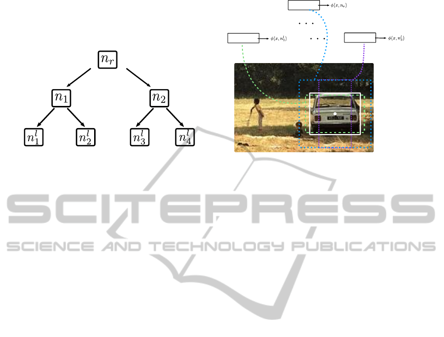
Figure 1: (a) We annotate the root filter by n
r
and the leaf filters by n
l
y
where y is its position from the left and corresponds
to a class. We also show the filter dimensions. The sizes for the leaf nodes are learned in as in (Felzenszwalb et al., ). The
parents’ nodes choose between the maximum height and width among their children’s dimensions. The attribute vector and
the final score for the ’car’ class is also depicted for an example. In (b), the example from (a) is used to show how the nodes
extract features around a center position x. The white bounding box indicates the ground truth annotation.
Let |T | be an arbitrary tree with k leaf nodes. Each
path to a leaf node models a class. n
i
.i ∈ {1, . . . , |T |}
designates any node in the tree and |T | is the total
number of leaf nodes. Further, n
r
and n
l
i
, i ∈ {1, . . . , k}
shall represent the root node and the i-th leaf node
as annotated in Fig. 1. anc(n
i
) is the set of the an-
cestors of node n
i
including itself and desc(n
i
) the
set of the descendants excluding n
i
. Each path to
node n
i
is determined by its attribute vector Λ
i
=
(λ
1
, . . . , λ
j
, . . . , λ
|T |
) ∈ R
|T |
with
λ
j
=
1 , if n
j
∈ anc(n
i
)
0 , otherwise
(1)
In other words, the entries λ
j
in the attribute vec-
tor are 1 for nodes lying on the path up to the node
n
i
and 0 otherwise (see Fig. 1). In addition, let x
be a position in an image. The feature vector φ
i
(x)
the features for node n
i
at the location x. As can be
seen in Fig. 1, every node extracts features around
a region centered by x. We refer to the concate-
nated vector of all the feature vectors from top-to-
bottom and left-to-right by Φ(x). The class labels
y
i
∈ Y ≡ {y
1
, . . . , y
k
, y
bg
} ≡ Y
+
∪ {y
bg
} are positive
for the target classes and negative y
bg
= −1 for the
background regions.
Every node represents a parameter vector w
i
de-
termined during training. They are filters attribut-
ing a partial score w
T
i
· φ
i
(x) to a location x. Finally,
let w = {w
r
, w
2
, . . . , w
|T |
} be the stacked vector of all
w(n
i
).
3.1 Our Object Detection Model
Given an input image, our objective is to locate ob-
jects belonging to the k target classes. We assign to
ever possible location in the image a label y
i
∈ Y
+
if
the object is an target object or y
i
= y
bg
if the region
is background.
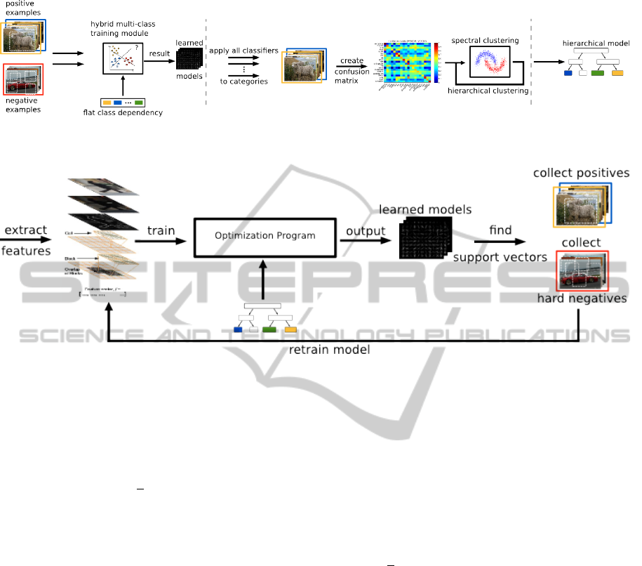
Our object detection process follows the follow-
ing pipeline as shown in Fig. 2. The input image is
scaled with different scaling factors to allow detecting
objects of various sizes. Next, features are extracted
for every scale. The grouping of all these features
across all levels is called a feature pyramid. We do
not limit our choice to a specific feature descriptor.
Here, we report our experiments on a variant of the
histogram of orientated gradients (HOG) (Dalal and
Triggs, 2005b) as proposed in (Felzenszwalb et al.,
2010) for its popularity and simplicity. Our hierar-
chical classifier attributes a score and label to every
location in the feature pyramid. For a positive re-
gion, there maybe several positive responding posi-
tions around that region. We merge all the overlap-
ping responses using a non-maxima suppression step
(see Sec. 3.2). The result is a set of possible instances
of the target objects.
Our detection module unifies classification and
ranking tasks. The objects in the feature pyramid are
ranked among the k target class. The class label is de-
termined by the highest scoring class. The object is
classified as background if the highest score is nega-
tive.
VISAPP2014-InternationalConferenceonComputerVisionTheoryandApplications
106
Input image
Feature extraction at one scale
NMS
Scaled images
Multi-class classifier
Output image
Figure 2: We use a sliding window approach to detect objects of different categories in still images. Our hierarchical detector
ranks and classifies between object categories and background.
3.2 Inference
For a given location x in the feature pyramid, we cal-
culate a score score(x) which is the best score pro-
duced by all the single classes:
score(x) = max
y∈{1,...,k}
score
y
(x) (2)
The object label ˆy is determined by :
ˆy =
−1 , if score(x) ≤ 0
argmax score(x) , otherwise
(3)
Next, let Φ
i
(x) define the concatenated feature vec-
tors of all the features φ
i
(x) extracted by each node
lying on the path to node n
i
. The features extracted
by nodes not being an ancestor of n
i
are zeroed. More
formally:
Φ
i
(x) = Λ
i
⊗ Φ(x) =
λ
1
· φ
r
(x)
λ
2
· φ
1
(x)
···
λ
|T |
· φ
l
k
(x)
(4)
This kind of representation allows to define classes
by local to global parameters as individual classes are
grouped together into global super-classes. Then, the
scoring function of a class y is given by:
score
y
(x) = w
T
· Φ
l
y
(x) (5)
The Eq. 5 is used in Eq. 3 and Eq. 2 to determine the
final class score and label of a position x in the feature
pyramid.
3.3 Non-maxima Suppression
We assume that object instances of the same class
cannot share the same location in an image. We sup-
press multiple instances using our non-maxima sup-
pression scheme (NMS). We treat every class sepa-
rately. For a given class, we sort all the scores in
decreasing order and reject the remaining detections
having a sufficient overlap (e.g. 0.5%) with the higher
scoring detections. Thus, we assure that same in-
stances do not share the same positions. Different ob-
ject categories can share nearby locations e.g. a per-
son and bicycle.
4 LEARNING THE
HIERARCHICAL TREE
MODEL
In this section, we describe our learning algorithm
which automatically learns the tree structure, the di-
mensions of the filters and the weight vectors of each
node in the tree in a joint hybrid framework.
4.1 Learning the Hierarchy
The tree T is built in an automatic way. The goal is
to hierarchically group similar classes. We say two
classes are similar if they are likely to be confused.
Grouping classes together allows to better general-
ize to future unseen examples as the super-classes
are trained using all the samples of its descendant
classes. For example a ’bicycle’ and a ’motorbike’
share many features and training a super-class node
{’bicycle’,’motorbike’} increases their discriminative
power.
We build a class similarity matrix S : k × k where
each element s
i j
measures the similarity between
class i and j. To this end, a detector is trained for
each class. The k detectors classify the objects of
all the other classes. The similarity s
i j
is the median
value given by classifying examples of class i with the
JointLearningforMulti-classObjectDetection
107
(a)
(b)
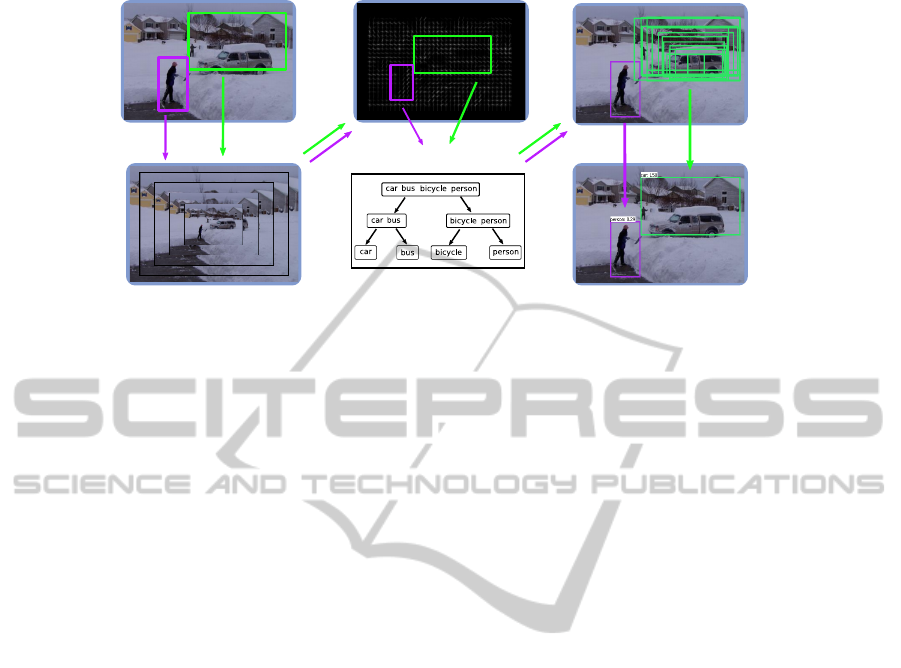
Figure 3: Illustating the different steps during the training process. (a) shows the creation of the hierarchy. The hybrid multi-
class training module is shown in (b). Given some training data, it extracts the features, trains the filters of the tree and if
necessary applies boostrapping to collect support vectors.
detection model of class j. To obtain a symmetrical
matrix, we average with its transposed:
S ←
1
2
(S + S
T
) (6)
Spectral clustering (Luxburg, 2007) is a clustering
technique which uses the spectrum of a similarity ma-
trix to partition the data. The objective is to build
(two) groups having a high intra-class but low inter-
class similarity. We apply spectral clustering hierar-
chically to S . At each iteration, the data is split into
two groups until the leaf nodes are reached. We en-
force balanced binary trees in the k-means step of the
spectral clustering algorithm. The result is the struc-
ture of our tree T . The tree building process is de-
picted in Fig. 3.
4.2 Problem Formulation
As described in Sec. 3, our hierarchical framework
ranks and classifies object regions. We use support
vector machines (SVM) to learn the weight vectors,
of each node in the tree. Traditional SVM solvers
as (Joachims, 1999; Chang and Lin, 2011) minimize
a max margin problem subject to classification con-
straints. Other solvers such as RankSVM (Joachims,
2002) or PRSVM (Chapelle and Keerthi, 2010) train
on ranking constraints where the goal is to rank the
correct class label higher than all the other classes.
We suggest a novel optimization problem consist-
ing of a mixture of classification and ranking con-
straints. Given n
+
positive and n
−
negative samples,
the problem is formulated as following:
min
w,ξ
i
( j)≥0
1
2
kwk
2
+C
n
+
∑
i=1
(ξ
i
+
n
+
∑
j=1
ξ
i j
) +
n
−
×n
+
∑
i, j
ξ
i j
!
(7a)
s.t. ∀y
i
∈ Y
+
, ∀y
j
∈ Y
+
: w
T
· δΦ
i
(y
j
) ≥ 1 − ξ
i j
(7b)
: w
T
· Φ
l
y
i
(x
i
) ≥ 1 − ξ
i
(7c)
∀y
i
∈ {y
bg
}, ∀y
j
∈ Y
+
: −w
T
· Φ
l
y
j
(x
i
) ≥ 1 − ξ
i j
,
(7d)
where δΦ
i
(y) = Φ
l
y
i
(x
i
) − Φ
l
y
(x
i
) and w a concatena-
tion of the filter weights in the tree T. The objective
function 7a minimizes two kinds of errors:
1.
n
+
∑
i=1
ξ
i
+
n
−
n
+
∑
i, j
ξ
i j
is the error of classifying target
regions as negative or classifying a background
sample as one of the k classes.
VISAPP2014-InternationalConferenceonComputerVisionTheoryandApplications
108

Algorithm 1: Learn weight vectors of each node in T .
1: Input: Tree T
2: Samples: {(x
1
, y
1
), . . . , (x
n
, y
n
)} ∈ X × Y
3: Output: w = {w
r
, . . . , w
|T |
}
4: W =
/
0
5: repeat
6: for all i = 1 . . . n do
7: ¯y
i
= argmax
y∈Y
+
1 + w
T
· Φ
l
y
(x
i
)
8: end for
9: W ←
1
n
{
∑
n
+
i=1
(w
T
· Φ
y
i
(x
i
)−
max(w
T
·Φ
¯y
i
(x
i
), 0) −
∑
n
−
i=1
w
T
·Φ
l
¯y
i
(x
i
)} ≥ 1 −
ξ
10: W → SVM
light
11: until stopping criteria is reached
2.
n
+
∑
j=1
ξ
i j
is the error of classifying an object of class
y
i
as y
j
.
7d and 7c represent the (n
+
+ n
−
) classification con-
straints where as 7b are the (n
+
× n
−
) ranking con-
straints. This makes a total of (n
+
× n
−
+ n
+
+ n
−
)
constraints which need to be optimized (Sec. 4.3).
4.3 Cutting-plane Optimization
The optimization problem in Eq. 7 is a convex op-
timization problem. We apply the cutting plane algo-
rithm (Joachims et al., 2009) to considerable speed-up
detection time. First, the n-slack formulation in Eq.
7 is rewritten as a 1-slack formulation, All the con-
straints share the same slack variable ξ thus giving us
the following learning task:
min
w,ξ≥0
1
2
kwk
2
+Cξ (8a)
s.t. ∀( ¯y
1
, · · · , ¯y
n
) ∈ Y
+
n
:
1
n
{
n
+
∑
i=1
(w
T
· δΦ
i
( ¯y) + w
T
· Φ
l
y
i
(x
i
))
−
n
−
∑
i=1
w
T
· Φ
l
¯y
(x
i
)} ≥ 1 − ξ.
(8b)
At the first sight, the formulation suffers from the
huge amount of constraints Y
n
namely one constraint
for each possible combination of labels (¯y
1
, · · · , ¯y
n
) ∈
Y
n
. The cutting plane algorithm only uses a small
subset of all possible constraints by iteratively build-
ing a working set W of constraints. At each iteration,
one constraint at a time is added to W . The cutting
plane optimization is summarized in Algorithm 1.
The algorithm starts with an empty working set
and a starting weight vector w. In line 7, the most
discriminative class label is calculated for each train-
ing sample. The label ¯y
i
is the class which confuses
most with the ground truth class. Line 9 adds the
new constraint into the working set. This constraint is
the sum of individual constraints producing only one
single new constraint per iteration. We use SVM
light
(Joachims, 1999) to solve the constraints in the work-
ing set.
4.4 Implementation Details
We changed the publicly available SVMStruct pack-
age (Joachims et al., 2009) to include our definition
of the joint feature vector and the combined con-
straints. The object descriptors are histogram of ori-
entated gradients (Felzenszwalb et al., 2010).
During training, we first learn the hierarchy. Us-
ing the tree, we train a model based on all posi-
tive samples and randomly collected negatives. This
model is iteratively used to collect high scoring neg-
ative samples called hard negatives. This bootstrap-
ping procedure strongly improves object detection
systems.
The nodes are characterized by a pair (v
i
, dim
i
).
v
i
is a vector specifying the location of the filter rel-
ative to the root position. dim
i
designates the dimen-
sions of node n
i
. These dimensions for every class are
built in a bottom-to-up fashion. First the dimensions
of the leaf filters are determined as in (Felzenszwalb
et al., ). The aspect ratio is chosen to be the most
common mode in the annotated bounding boxes. The
size is picked up not to be larger than 80% of the data.
Given the width and height of each node, the dimen-
sions of the remaining nodes are the maximum width
W
i
respectively height H
i
over its children dimensions
(refer to Fig. 1 for an example):
W
i
= max
n
j
∈desc(n
i
)
W
j
H
i
= max
n
j
∈desc(n
i
)
H
j
(9)
5 EXPERIMENTAL RESULTS
The following section shows the evaluations of our
approach on the PASCAL VOC’07 (Everingham
et al., ) dataset and protocol. The dataset has a to-
tal of 20 classes represented by 12608 annotated ob-
jects. It is equally divided into a training and valida-
tion set. We study and illustrate (1) the importance
of hierarchy to increase multi-class object detection
performance which is the main contribution of this
work and (2) the ability to generalize fast when using
our tree. We use simple HOG features to show our
contribution. As such, our results are relative to the
performance of HOG and should not be compared to
JointLearningforMulti-classObjectDetection
109

state-of-the-art object detectors. More powerful fea-
tures could have been used. We opted for HOG for its
popularity and widespread usage.
Detection Models. Our method is tested on five de-
signed detection algorithms which allow to validate
the different aspects of our method : (1) One-vs-
All (OvA) treats every class separately. It trains an
SVM for each class. The final decision functions are
transformed into a probabilistic output using (Platt
et al., 2000). (2) The second model called ’ours flat’
learns all the weight vectors jointly using the hybrid
learning algorithm but no hierarchical structure. The
last model ’ours tree’ trains a complete hierarchical
model using the combination of ranking and classifi-
cation constraints.
Detection Performance. The goal is to show how
the hierarchical structure optimized using the hybrid
training algorithm improves detection performance.
We evaluate on 5 different settings by varying the
number of classes k = {2, 4, 6, 8, 10} and show that
the improvement is true independent of k. The 10
selected classes are: {’bus’, ’bicycle’, ’motorbike’,
’car’, ’aeroplane’, ’person’, ’cow’, ’horse’, ’dog’,
’cat’}. Among the classes are certain ones where
we would expect a strong degree of feature sharing
(e.g.’car’ and ’bus’) and other categories with less
common properties (e.g.’person’ and ’aeroplane’).
Table 1 illustrates the detection performance of the
detection models for the different settings (k) in terms
of the mean average precision (mAP) used in PAS-
CAL VOC’07 evaluation protocol. The tree structure
for k = 10 classes with the corresponding similarity
matrix used to deduce the tree is depicted in Fig. 5.
’ours flat’ achieves slightly better results compared to
OvA. A joint learning of all filters and mixing clas-
sification and ranking constraints achieve at least as
good results as OvA. Using our complete algorithm
’ours tree’ which uses a tree yields the best results.
This is due to an increase of the number of linear fil-
ters used for the final classification and the feature
sharing between neighboring nodes.
The individual scores for k = 10 are depicted in
table 2. 8 out of 10 classes improve in performance
compared to OvA using our joint learning framework.
Only 2 classes {’bus’,’dog’} degrade in performance.
The classes ’car’ (+3.1) and bicycle (+5.9) have the
best increase in performance.
Fast Generalizing Ability. We learn a model rep-
resenting the classes {’bicycle’,’motorbike’} using
OvA and our hierarchical detector. We investigate
how quickly the average precision (AP) of class ’mo-
torbike’ achieves its maximum score when we vary
the number of its training examples. The intuition be-
Table 1: Mean average precision (mAP) of the 4 detection
models. Our hierarchical approach always improves over
OvA.
k 2 4 6 8 10
OvA 24.1 23.4 20.6 18.3 15.2
ours flat 24.4 23.9 20.7 18.8 15.5
ours tree 25.5 25.7 23.6 20.6 16.4
hind this setup is to understand how the knowledge
of class ’bicycle’ helps to quickly learn the similar
class ’motorbike’. This comes close to transfer learn-
ing techniques (e.g. (Aytar and Zisserman, 2011; Lim
et al., 2011)) aiming at learning a new class with as
few examples as possible. Here, the class ’bicycle’
using all of its examples helps the class ’motorbike’
having fewer examples but highly similar features and
examples.
In Fig. 4, we illustrate the relative average preci-
sion of class ’bicycle’ using these two techniques in
function of the relative percentage of examples used.
We normalize all the AP to the AP when full examples
are available for both classes. We note that for OvA,
having very few training examples only 40% of the
final score is reached. However, using the hierarchi-
cal classifier, even with very few training examples,
nearly the full AP is attained. Our approach is able to
generalize fast when a small amount of samples are
available. This is due to the fact that these two classes
have may features and examples in common.
6 CONCLUSIONS
We presented a novel hierarchical multi-class detec-
tion system. Our approach is not limited to the
choice of the object descriptors. We combined rank-
ing and classification constraints giving a new op-
timization problem. Foreground objects are ranked
among each other while being able to classify fore-
ground/background regions. We learn the model in
a joint framework where we first learn the hierarchy
between objects and the train all the weight vectors
jointly.
The experimental results clearly showed an in-
crease of detection performance for different set-
tings in the number of classes. This is due to the
increased number of discriminative weight vectors
learned. Moreover, similar classes share features and
examples which help to generalize faster. This was
further illustrated in our experiments where having
few samples for one class still allowed to achieve the
score when the full training set is available.
In the future, we would like to enhance our hierar-
VISAPP2014-InternationalConferenceonComputerVisionTheoryandApplications
110
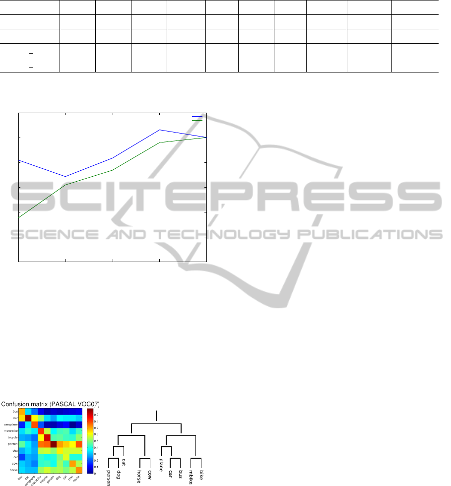
Table 2: Mean average precision for each class after learning k = 10 classes.
class aero bike bus car cat cow dog horse mbike person
#samples 306 353 229 1250 376 259 510 362 339 4690
OvA 17.6 20.3 24.0 29.2 2.3 8.4 3.1 14.4 15.3 17.5
ours flat 17.9 24.6 21.8 26.2 6.0 8.2 4.5 12.1 15.6 18.1
ours tree 20.3 26.2 21.5 32.3 2.3 11.4 1.2 15.4 15.5 18.2
0
0.2
0.4
0.6
0.8
1
1.2
0.2 0.4 0.6 0.8 1
Percentange of used samples
Learning with Few Samples
OvA
Hierarchy
Relative AP
Figure 4: The generalization ability of our approach. We
train a model for two classes {’motorbike’,’bicycle’} with
OvA and with our algorithm. We vary the number of ex-
amples and analyze the influence on the AP compared to
the AP when all the examples are available. OvA slowly
increases in performance as the number of examples in-
creases. Our approach achieves much faster its final AP
score. We noted a slightly better AP when using 80% of the
dataset. We believe that using all the samples introduces
more noise in the training process shifting the separating
decision line.
(a) (b)
Figure 5: (a) The similarity matrix S obtained for k = 10
classes when building the taxonomy. (b) The resulting tree
structure derived by the similarity matrix S .
chy with the deformable part model of (Felzenszwalb
et al., ). This new hierarchical deformable part model
allows us to automatically find parts between object
classes and understand its role to improve object de-
tection performance.
REFERENCES
Aytar, Y. and Zisserman, A. (2011). Tabula rasa: Model
transfer for object category detection. In IEEE Inter-
national Conference on Computer Vision.
Bengio, S., Weston, J., and Grangier, D. (2010). Label em-
bedding trees for large multi-class tasks. In NIPS.
Cai, L. and Hofmann, T. (2004). Hierarchical document
categorization with support vector machines. CIKM.
Chang, C.-C. and Lin, C.-J. (2011). LIBSVM: A library for
support vector machines. ACM Transactions on Intel-
ligent Systems and Technology. Software available at
http://www.csie.ntu.edu.tw/∼cjlin/libsvm.
Chapelle, O. and Keerthi, S. S. (2010). Efficient algorithms
for ranking with svms. Inf. Retr.
Choi, M. J., Torralba, A., and Willsky, A. S. (2012). Context
models and out-of-context objects. Pattern Recogni-
tion Letters.
Dalal, N. and Triggs, B. (2005a). Histograms of oriented
gradients for human detection. In CVPR.
Dalal, N. and Triggs, B. (2005b). Histograms of oriented
gradients for human detection. In International Con-
ference on Computer Vision & Pattern Recognition.
Dekel, O., Keshet, J., and Singer, Y. (2004). Large margin
hierarchical classification. In ICML.
Desai, C., Ramanan, D., and Fowlkes, C. (2011). Discrimi-
native models for multi-class object layout. IJCV.
Everingham, M., Van Gool, L., Williams, C. K. I., Winn,
J., and Zisserman, A. The PASCAL Visual Object
Classes Challenge 2007 (VOC2007) Results. http://
www.pascal-network.org/ challenges/ VOC/ voc2007/
workshop/index.html.
Felzenszwalb, P. F., Girshick, R. B., McAllester, D., and
Ramanan, D. Object detection with discriminatively
trained part based models. PAMI.
Felzenszwalb, P. F., Girshick, R. B., McAllester, D. A., and
Ramanan, D. (2010). Discriminative latent variable
models for object detection. In ICML.
Fidler, S., Boben, M., and Leonardis, A. (2010). A coarse-
to-fine taxonomy of constellations for fast multi-class
object detection. In ECCV.
Fidler, S. and Leonardis, A. (2007). Towards scalable repre-
sentations of object categories: Learning a hierarchy
of parts. In CVPR.
Gao, T. and Koller, D. (2011). Discriminative learning of
relaxed hierarchy for large-scale visual recognition. In
ICCV.
Griffin, G. and Perona, P. (2008). Learning and using tax-
onomies for fast visual categorization.
JointLearningforMulti-classObjectDetection
111

Joachims, T. (1999). Advances in kernel methods. chapter
Making large-scale support vector machine learning
practical.
Joachims, T. (2002). Optimizing search engines using click-
through data. In KDD.
Joachims, T., Finley, T., and Yu, C.-N. (2009). Cutting-
plane training of structural svms. Machine Learning.
Joshua B. Tenenbaum1, Charles Kemp, T. L. G. N. D. G.
(2011). How to grow a mind: Statistics, structure, and
abstraction. Science.
Kressel, U. H.-G. (1999). Advances in kernel methods.
chapter Pairwise classification and support vector ma-
chines.
Lim, J. J., Salakhutdinov, R., and Torralba, A. (2011).
Transfer learning by borrowing examples for multi-
class object detection. In Neural Information Process-
ing Systems (NIPS).
Luxburg, U. (2007). A tutorial on spectral clustering. Statis-
tics and Computing.
Marszalek, M. and Schmid, C. (2008). Constructing cate-
gory hierarchies for visual recognition. In ECCV.
Opelt, A., Pinz, A., and Zisserman, A. (2008). Learning
an alphabet of shape and appearance for multi-class
object detection. IJCV.
Ott, P. and Everingham, M. (2011). Shared parts for de-
formable part-based models. In CVPR.
Platt, J. C., Cristianini, N., and Shawe-taylor, J. (2000).
Large margin dags for multiclass classification.
Razavi, N., Gall, J., and Gool, L. J. V. (2011). Scalable
multi-class object detection. In CVPR.
Salakhutdinov, R., Torralba, A., and Tenenbaum, J. B.
(2011). Learning to share visual appearance for mul-
ticlass object detection. In CVPR.
Torralba, A., Murphy, K. P., and Freeman, W. T. (2004).
Sharing features: efficient boosting procedures for
multiclass object detection. In CVPR.
Torralba, A., Murphy, K. P., and Freeman, W. T. (2007).
Sharing visual features for multiclass and multiview
object detection. PAMI.
Tsochantaridis, I., Hofmann, T., Joachims, T., and Altun, Y.
(2004). Support vector machine learning for interde-
pendent and structured output spaces. In ICML.
Xiao, L., Zhou, D., and Wu, M. (2011). Hierarchical clas-
sification via orthogonal transfer. In ICML.
Zhang, J., Huang, K., Yu, Y., and Tan, T. (2011). Boosted
local structured hog-lbp for object localization. In
CVPR.
Zhu, L., Chen, Y., Torralba, A., Freeman, W. T., and Yuille,
A. L. (2010). Part and appearance sharing: Recursive
compositional models for multi-view. In CVPR.
VISAPP2014-InternationalConferenceonComputerVisionTheoryandApplications
112
